Maclaurin Series for the Cosine Function

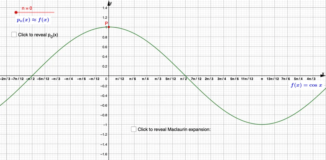
This GeoGebra example demonstrates the Maclaurin series approximation of the cosine function cos(x), showing how successive polynomial terms converge to the original curve near the origin. Core mathematical concepts include Taylor and Maclaurin series, trigonometric functions, polynomial approximation, convergence, and real-valued function graphing. The construction relies on GeoGebra's Point command to generate points P_0 through P_{10}, together with function f and text labels text1 through text14 to display each approximation stage and its coefficients; objects A, a, and b control parameters such as expansion order and viewing window. It is suitable for high school advanced mathematics and university calculus courses, ideal for teaching power series expansion, function approximation, and numerical analysis visualization.