Lotka–Volterra Predation Model: Slope Field and Phase-Plot from Numerical ODE So

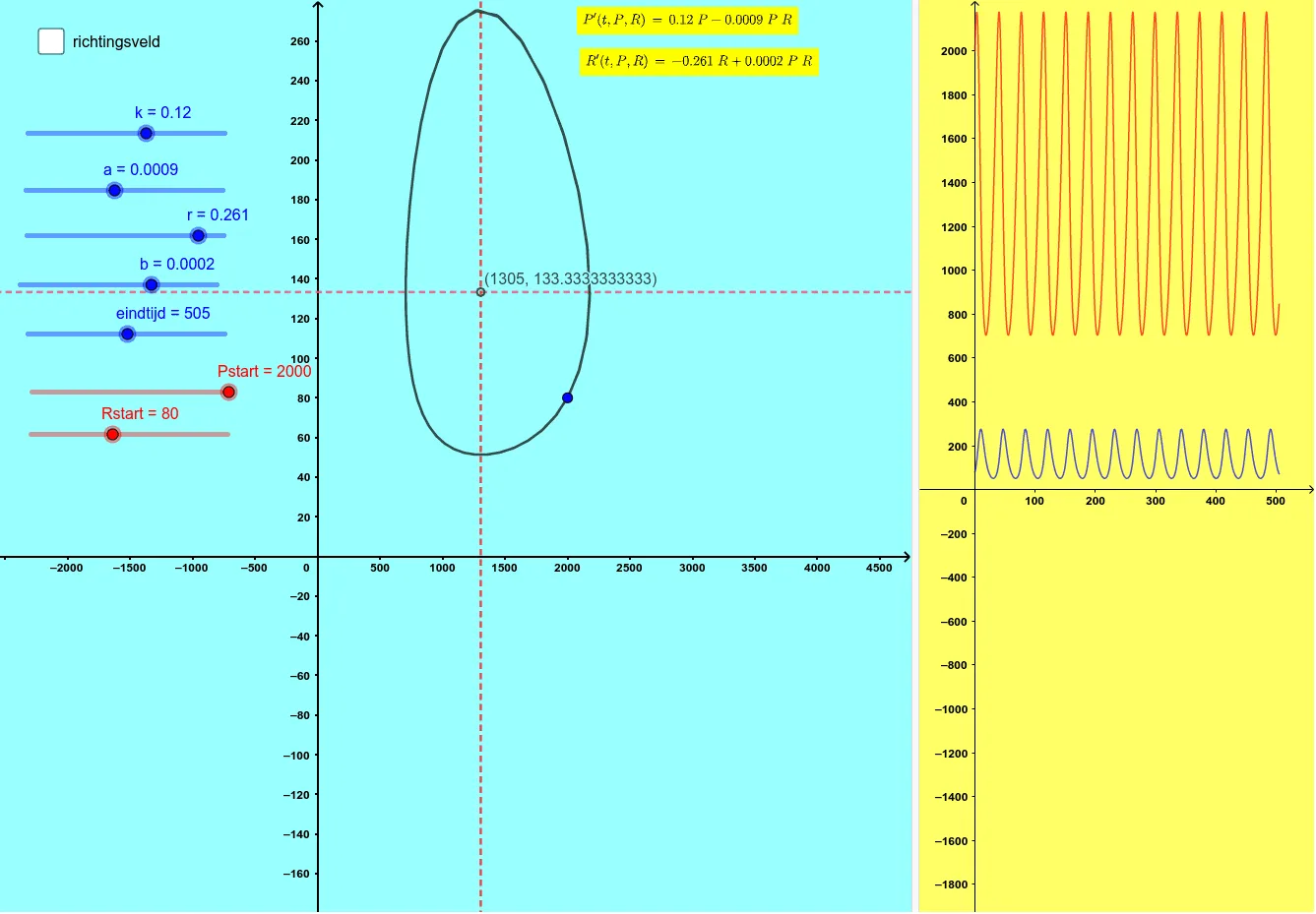
This example demonstrates how the Lotka–Volterra predator–prey system evolves over time by combining a slope field (direction field) with a phase plot. You can see local solution tendencies from the slope field and then observe the global orbit structure in the phase plane. The key mathematics includes modeling with ordinary differential equations, solving ODEs numerically, constructing direction fields, and interpreting phase trajectories. In GeoGebra, construction relies on NSolveODE, SolveODE, and LaTeX to define and compute solutions, SlopeField to generate the direction field, and faseplot to plot the resulting phase portrait. Parameters (e.g., k, a, b, r, dt, and other constants) and initial conditions (Pstart, Rstart) drive the dynamics. Supporting objects such as numeriekeIntegraal1/2, richtingsveld (vector/direction field), and auxiliary functions like f and vgl1 are used to visualize the model and annotate outcomes (tekst1/tekst2). Suitable for advanced high school through undergraduate study in calculus and differential equations, especially for topics like numerical integration, dynamical systems, and population modeling.