Lorentz Transformation Visualization

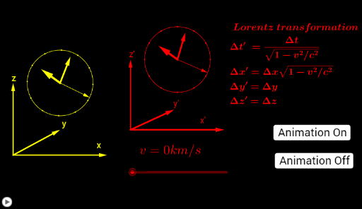
This GeoGebra example dynamically illustrates the Lorentz transformation from special relativity, representing the linear transformation of spacetime coordinates through geometric elements such as vectors, circles, and rotations. The core mathematical concepts include linear transformations, hyperbolic geometry, light-cone structure, and relativistic effects like time dilation and length contraction. The construction uses the Vector command to create pre- and post-transformation vectors, Dilate for scaling, Circle and Rotate to exhibit rotational symmetry, Sequence to generate point series, and a slider parameter γ (Lorentz factor) to adjust the transformation strength interactively. Suitable for high school to university-level physics or mathematics instruction, this example helps students grasp the essence of coordinate changes in Minkowski spacetime and serves as an extension case combining analytic geometry with linear algebra.