
Parallel Vector Transport
Loading the math board and drawing, please wait…
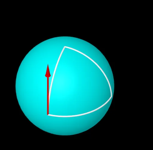
This example demonstrates the concept of parallel vector transport in geometric contexts, involving derivatives, geometric means, and isosceles triangles. The construction uses GeoGebra commands like Sphere, Segment, If, and Line to visualize the vectors and their properties. Suitable for high school students learning geometry and calculus fundamentals.
GeoGebra Commands & Parameters
Sphere((0, 0), 1) → aSegment((1, 0, 0), (1, 0, 1)) → uIf(b > 0 ∧ b < π / 2, Rotate[u, (-b), yAxis]) → u'If(b > π / 2 ∧ b ≤ π, Rotate[u', (-(b - π / 2)), xAxis]) → u''Line((1, 0, 0), (1, 0, 1)) → eIf(b > 0 ∧ b > π / 2, Rotate[e, (-b), yAxis]) → e'If(b > π / 2 ∧ π ≤ π, Rotate[e', (-(b - π / 2)), xAxis]) → e''If(b > π ∧ b < (3 / 2 * π), Rotate[e'', (-(b - π)), zAxis]) → e'''Point(e''') → APoint(e) → BCircleArc((0, 0, 0), (1, 0, 0), (0, 0, 1), xOyPlane) → fCircleArc((0, 0, 0), (0, 1, 0), (0, 0, 1), xOyPlane) → gCircleArc((0, 0, 0), (1, 0, 0), (0, 1, 0), xOyPlane) → hIf(b > π ∧ b < (3 / 2 * π), Rotate[u'', (-(b - π)), zAxis]) → u'''Point(u''') → DAngle(B, C, D) → αCircle((1, 0, 0), 0.05, xOyPlane) → cTranslate(c, Vector[(0, 0, 0), (0, 0, 1)]) → c'Cone(c', 0.3) → d, k, iIf(b ≤ π / 2, Rotate[i, (-b), yAxis]) → jIf(b > π / 2 ∧ b ≤ π, Rotate[j, (-(b - π / 2)), xAxis]) → lIf(b < π / 2, Rotate[d, (-b), yAxis]) → mIf(b ≥ π / 2 ∧ b < π, Rotate[m, (-(b - π / 2)), xAxis]) → nIf(b > π, Rotate[n, (-(b - π)), zAxis]) → oRotate(c, ((-π)) / 2, xAxis) → c'_1Rotate(c'_1, π / 2, zAxis) → pCone(p, 0.3) → q, r, sTranslate(q, Vector[(0, 0, 0), (-1, 0, 0)]) → g'Rotate(g', π / 2, xAxis) → g''If(b > π / 2 ∧ b < π, Rotate[g'', (-(b - π / 2)), xAxis]) → tIf(b > π ∧ b < (1.5 * π), Rotate[g', (-(b - π)), zAxis]) → v