
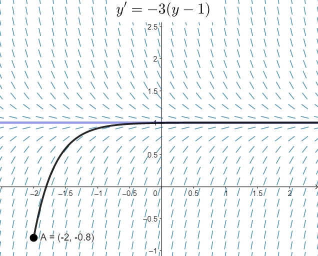
Long term behaviour of differential equations
Loading the math board and drawing, please wait…
In collections
MATH1052-edX
This example demonstrates the long-term behavior of differential equations using parallelograms and secant lines. Key mathematical concepts include differential equations, secant lines, real numbers, and polynomial functions. Construction involves GeoGebra commands like SlopeField and SolveODE, with objects such as yA, button1, A, f, a, F, Sol1, h, text1. Suitable for high school or university mathematics courses to understand dynamic properties of differential equations.
GeoGebra Commands & Parameters
SlopeField(f, 25, 0.7) → FSolveODE(f, x(A), y(A), 10, 0.01) → Sol1
AI Drawing Prompt Reference
Draw a graph showing the long-term behavior of a differential equation. First, depict the slope field for a polynomial function using dense slope indicators across a region of the coordinate plane. Then, starting from an initial point, plot the solution curve of the differential equation, demonstrating how the solution evolves over time and approaches its asymptotic behavior, helping viewers understand the dynamic properties and long-term trends of the differential equation.
The prompt above was compiled from the original drawing commands and is for reference only.