Local Extrema via Tangent Lines: Geometric Insight

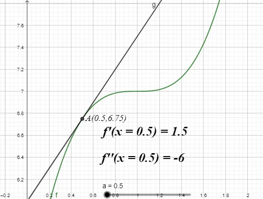
This example illustrates how local extrema of a function can be visualized by selecting key points on the graph and examining the corresponding tangent-line behavior. The geometric phenomenon is linked to the calculus idea that the derivative relates to the slope of the tangent line, helping students understand why local maxima/minima occur where the slope is zero and how tangent characteristics change around those points. Core math concepts include differential calculus, local extrema (local maximum/minimum), the geometric meaning of the derivative, and point-based reasoning using selected x-values and auxiliary reference objects. Construction-wise, the provided GeoGebra script emphasizes the commands Tangent and Text: for the function f and selected points (a, A, g, b, c), it draws tangents and uses multiple text objects (text1, text2, text3) to label the critical locations and the inferred extremum-related conclusions. Suitable for high-school (Class XII) calculus instruction, classroom demonstrations, and guided practice on derivatives and extremum interpretation.