Geometric Demonstration of Lagrange Multipliers: Tangency of Level Curves and Co

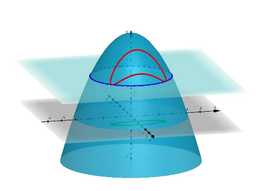
This example demonstrates the geometric principle of Lagrange multipliers: the local extreme points of a function f(x,y) subject to constraint g(x,y)=k occur at points where the level curves of f are tangent to the constraint curve. Using GeoGebra, the level curves of the objective function and the constraint curve are drawn; CurveCartesian generates the curves while IntersectPath finds their intersection points. This visualization clearly shows the relationship between the gradient direction and the normal vector of the constraint curve. Suitable for calculus and optimization courses in higher education.