Explaining Derivatives with Tangents and Geometry for Area–Perimeter Optimizatio

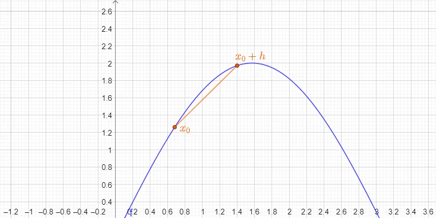
This GeoGebra example demonstrates how derivatives (via tangent slopes) can be used to interpret and solve optimization problems using geometric quantities. By constructing key points on graphs/functions and drawing tangents at selected locations, it highlights that the derivative encodes the instantaneous rate of change, which then guides the search for optimal configurations under geometric constraints. The example’s core concepts include calculus (derivative interpretation through tangents), function behavior, and optimization using area/perimeter-style measures. Construction-wise, the setup is driven by commands Point, Tangent, and Segment, creating objects such as f, g, h together with corresponding labeled points (e.g., A, B, C) and segments that form the geometric structure used for reasoning. Suitable for advanced high school through early undergraduate calculus and applications (including modeling in production economics or constrained optimization lessons).