
Lissajous Curve and Sine Function
Loading the math board and drawing, please wait…
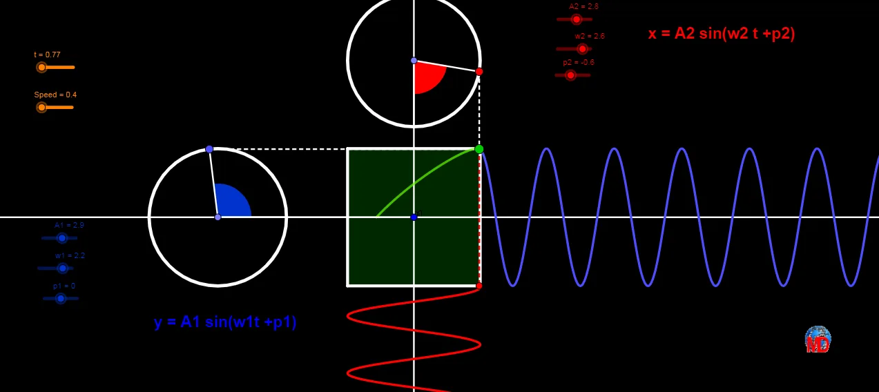
This example demonstrates how Lissajous curves are generated by the addition of sine functions. Key math concepts include sine functions, trigonometry, parametric equations, and coordinate geometry. Construction highlights involve commands/objects like Polygon, CurveCartesian, Line, Point, Circle, Intersect, Rotate, Segment, Angle, and Translate from GeoGebra. Suitable for high school mathematics teaching to understand the叠加 and transformation patterns of function graphs.
GeoGebra Commands & Parameters
Polygon(E, D, B, C) → q1, e, d, b, cCurveCartesian(x(O) + (A2 * sin((w2 * k) + p2)), y(O) + (A1 * sin((w1 * k) + p1)), k, 0, t) → aLine(O, yAxis) → fLine(O, xAxis) → gPoint(f) → FPoint(g) → GCircle(F, A2, xOyPlane) → hCircle(G, A1, xOyPlane) → pIntersect(f, h) → L, MRotate(M, (w2 * t) + p2, F) → M'Segment(M', A) → iSegment(F, M') → lIntersect(g, p) → H, IRotate(H, (w1 * t) + p1, G) → H'Segment(G, H') → jSegment(H', A) → mSegment(G, H) → nSegment(F, M) → qAngle(M, F, M', xOyPlane) → αAngle(H, G, H', xOyPlane) → βSegment(G, O) → f_1Line(G, O) → h_1Line(F, O) → g_1CurveCartesian(((-A2) * sin((w2 * i) - p2 - (w2 * t))), i, i, (-6 * π), 0) → kTranslate(s, Vector[O, O + (A2, 0)]) → s_{1}Line(A, f_1) → i_1Intersect(i_1, d) → JSegment(A, J) → j_1Line(A, q) → k_1Intersect(e, k_1) → KTranslate(k, Vector[O, O - (0, A1)]) → k'Segment(A, K) → l_1
AI Drawing Prompt Reference
Draw a Lissajous curve and sine function graph. Start by drawing a unit circle and the x-axis and y-axis. Then, generate two circles by rotating and moving, and calculate their intersection points. Use these points and the origin to construct the parametric equation of the Lissajous curve. Finally, add angle markings and auxiliary lines to demonstrate the curve generation process.
The prompt above was compiled from the original drawing commands and is for reference only.