
Lemniscate Polar Equation Graphing
Loading the math board and drawing, please wait…
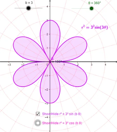
This example demonstrates the shape of a lemniscate defined by polar equations r²=a²*cos(b*θ) or r²=a²*sin(b*θ). It involves core math concepts like polar coordinates, trigonometric functions, parametric equations, and curve sketching. The construction uses GeoGebra commands such as CurveCartesian, Point, Angle, and Line. It is suitable for high school mathematics education to understand the relationship between polar coordinate equations and curve shapes, as well as the effect of parameters on the graph.
GeoGebra Commands & Parameters
CurveCartesian((r1(i) * cos(i)), (r1(i) * sin(i)), i, 0, θ) → b1Point(b1) → AAngle((1, 0), A, B) → αCurveCartesian(cos(i), sin(i), i, 0, 6.283185307179586) → cLine((0, 0), (1, 1)) → eLine((0, 0), (1, 1.7320508075688772)) → fLine((0, 0), (1.7320508075688772, 1)) → gLine((0, 0), (-1.73205, 1)) → hLine((0, 0), (1, -1.73205)) → iLine((0, 0), (1, -1)) → jLine((0, -0.02), (0.9659258262890683, 0.23881904510252072)) → kLine((0, 0), (0.25881904510252074, 0.9659258262890683)) → lLine((0, -0.02), (-0.25881904510252085, 0.9659258262890683)) → mLine((0, -0.02), (-0.9659258262890682, 0.258819045102521)) → nCurveCartesian((2 * cos(i)), (2 * sin(i)), i, 0, 6.28319) → oCurveCartesian((3 * cos(i)), (3 * sin(i)), i, 0, 6.28319) → pCurveCartesian((4 * cos(i)), (4 * sin(i)), i, 0, 6.28319) → qCurveCartesian((5 * cos(i)), (5 * sin(i)), i, 0, 6.28319) → sCurveCartesian((6 * cos(i)), (6 * sin(i)), i, 0, 6.28319) → tCurveCartesian((7 * cos(i)), (7 * sin(i)), i, 0, 6.28319) → uCurveCartesian((r2(i) * cos(i)), (r2(i) * sin(i)), i, 0, θ) → bCurveCartesian((v1(i) * cos(i)), (v1(i) * sin(i)), i, 0, θ) → rCurveCartesian((v2(i) * cos(i)), (v2(i) * sin(i)), i, 0, θ) → vLine(A, B) → dLine(D, E) → a_1
AI Drawing Prompt Reference
Graph the lemniscate defined by polar equations r²=a²*cos(b*θ) or r²=a²*sin(b*θ), showing how parameters a and b affect the shape. Start by plotting polar curves, then add reference lines, angles, and concentric circles of varying sizes to illustrate the impact of parameter changes, emphasizing the relationship between polar and Cartesian coordinates.
The prompt above was compiled from the original drawing commands and is for reference only.