
Linear Regression with Random Data Set
Loading the math board and drawing, please wait…
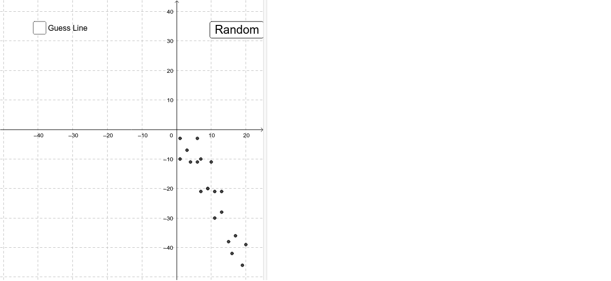
This example demonstrates linear regression analysis using a randomly generated set of data points. Key math concepts include linear regression, data fitting, and statistical probability. GeoGebra commands and objects used in the construction are Random (for point generation), Line (for drawing lines), Intersect (for intersection calculations), Polygon (for polygons), Vector (for vectors), RSquare (for coefficient of determination), SampleSD (for sample standard deviation), Median (for median calculation), FitLineY (for fitting a line), Circle (for circles), and Text (for annotations). Suitable for high school mathematics or statistics courses, teaching linear regression models and data visualization.
GeoGebra Commands & Parameters
Random(1, 20) → A2Random(1, 20) → A1Random(1, 20) → A3Random(1, 20) → A4Random(1, 20) → A5Random(1, 20) → A6Random(1, 20) → A7Random(1, 20) → A8Random(1, 20) → A9Random(1, 20) → A10Random(1, 20) → A11Random(1, 20) → A12Random(1, 20) → A13Random(1, 20) → A14Random(1, 20) → A15Random(1, 20) → A16Random(1, 20) → A17Random(1, 20) → A18Random(1, 20) → A19Random(1, 20) → A20Random(-2, 2) → slope_1Line(U, V) → line_{guess}Line(A, x = 0) → aLine(B, x = 0) → bLine(C, x = 0) → cLine(D, x = 0) → dLine(E, x = 0) → eLine(F, x = 0) → fLine(G, x = 0) → gLine(H, x = 0) → hLine(I, x = 0) → iLine(J, x = 0) → jLine(K, x = 0) → kLine(L, x = 0) → lLine(M, x = 0) → mLine(N, x = 0) → nLine(NP, x = 0) → npLine(O, x = 0) → pLine(P, x = 0) → qLine(R, x = 0) → sLine(S, x = 0) → tIntersect(line_{guess}, a) → A'Intersect(line_{guess}, b) → B'Intersect(line_{guess}, c) → C'Intersect(line_{guess}, d) → D'Intersect(line_{guess}, e) → E'Intersect(line_{guess}, f) → F'Intersect(line_{guess}, g) → G'Intersect(line_{guess}, h) → H'Intersect(line_{guess}, i) → I'Intersect(line_{guess}, j) → J'Intersect(line_{guess}, k) → K'Intersect(line_{guess}, l) → L'Intersect(line_{guess}, m) → M'Intersect(line_{guess}, n) → N'Intersect(line_{guess}, np) → NP'Intersect(line_{guess}, p) → O'Intersect(line_{guess}, q) → P'Intersect(line_{guess}, s) → R'Intersect(line_{guess}, t) → S'Line(Q, x = 0) → rIntersect(line_{guess}, r) → Q'Polygon(A', A, 4) → poly1, a_1, b_1, c_1, d_1, T, WPolygon(B', B, 4) → poly2, e_1, f_1, g_1, h_1, Z, A_1Polygon(D', D, 4) → poly3, i_1, j_1, k_1, l_1, B_1, C_1Polygon(E', E, 4) → poly4, m_1, n_1, p_1, q_1, D_1, E_1Polygon(C', C, 4) → poly5, r_1, s_1, t_1, a_2, F_1, G_1Polygon(F', F, 4) → poly6, b_2, c_2, d_2, e_2, H_1, I_1Polygon(G', G, 4) → poly7, f_2, g_2, h_2, i_2, J_1, K_1Polygon(H', H, 4) → poly8, j_2, k_2, l_2, m_2, L_1, M_1Polygon(I', I, 4) → poly9, n_2, p_2, q_2, r_2, N_1, O_1Polygon(J', J, 4) → poly10, s_2, t_2, a_3, b_3, P_1, Q_1Polygon(K', K, 4) → poly11, c_3, d_3, e_3, f_3, R_1, S_1Polygon(L', L, 4) → poly12, g_3, h_3, i_3, j_3, T_1, U_1Polygon(M', M, 4) → poly13, k_3, l_3, m_3, n_3, V_1, W_1Polygon(N', N, 4) → poly14, p_3, q_3, r_3, s_3, Z_1, A_2Polygon(NP', NP, 4) → poly15, t_3, a_4, b_4, c_4, B_2, C_2Polygon(P', P, 4) → poly16, d_4, e_4, f_4, g_4, D_2, E_2Polygon(O', O, 4) → poly17, h_4, i_4, j_4, k_4, F_2, G_2Polygon(Q', Q, 4) → poly18, l_4, m_4, n_4, p_4, H_2, I_2Polygon(R', R, 4) → poly19, q_4, r_4, s_4, t_4, J_2, K_2Polygon(S', S, 4) → poly20, a_5, b_5, c_5, d_5, L_2, M_2Vector((x(A), 0), (x(A), y(A) - y(A'))) → V_AVector((x(B), 0), (x(B), y(B) - y(B'))) → V_BVector((x(C), 0), (x(C), y(C) - y(C'))) → V_CVector((x(D), 0), (x(D), y(D) - y(D'))) → V_DVector((x(E), 0), (x(E), y(E) - y(E'))) → V_EVector((x(F), 0), (x(F), y(F) - y(F'))) → V_FVector((x(G), 0), (x(G), y(G) - y(G'))) → V_GVector((x(H), 0), (x(H), y(H) - y(H'))) → V_HVector((x(I), 0), (x(I), y(I) - y(I'))) → V_IVector((x(J), 0), (x(J), y(J) - y(J'))) → V_JVector((x(K), 0), (x(K), y(K) - y(K'))) → V_KVector((x(L), 0), (x(L), y(L) - y(L'))) → V_LVector((x(M), 0), (x(M), y(M) - y(M'))) → V_MVector((x(N), 0), (x(N), y(N) - y(N'))) → V_NVector((x(NP), 0), (x(NP), y(NP) - y(NP'))) → V_{NP}Vector((x(P), 0), (x(P), y(P) - y(P'))) → V_PVector((x(Q), 0), (x(Q), y(Q) - y(Q'))) → V_QVector((x(R), 0), (x(R), y(R) - y(R'))) → V_RVector((x(O), 0), (x(O), y(O) - y(O'))) → V_OVector((x(S), 0), (x(S), y(S) - y(S'))) → V_SRSquare(data, line_{guess}) → StrengthSampleSD(list_y) → SD_yMedian(list_x) → Median_xFitLineY(data) → line_{actual}Circle(((Median_x * 1.5), (2 * SD_y)), (Strength * Max[list_y] / 6)) → CorrelationCircleCircle(((Median_x * 1.5), (2 * SD_y)), (Strength * Max[list_y] / 6)) → CorrelationCircle_1Random(-10, 10) → yint_1Vector((Min[list_x] - 2, 0), (Min[list_x] - 2, over)) → Vector_{over}Vector((Min[list_x] - 2, 0), (Min[list_x] - 2, (-under))) → Vector_{under}Text(((Strength * 100) * "%"), (Max[list_x] + 2, 0)) → text1
AI Drawing Prompt Reference
Create a scatter plot using a randomly generated set of data points. Fit a line to these points to demonstrate linear regression. Draw several vertical lines from each point to the x-axis and label the values at the intersections. Include statistical annotations like the title and axis labels.
The prompt above was compiled from the original drawing commands and is for reference only.