Linear Inequalities Slider Demo

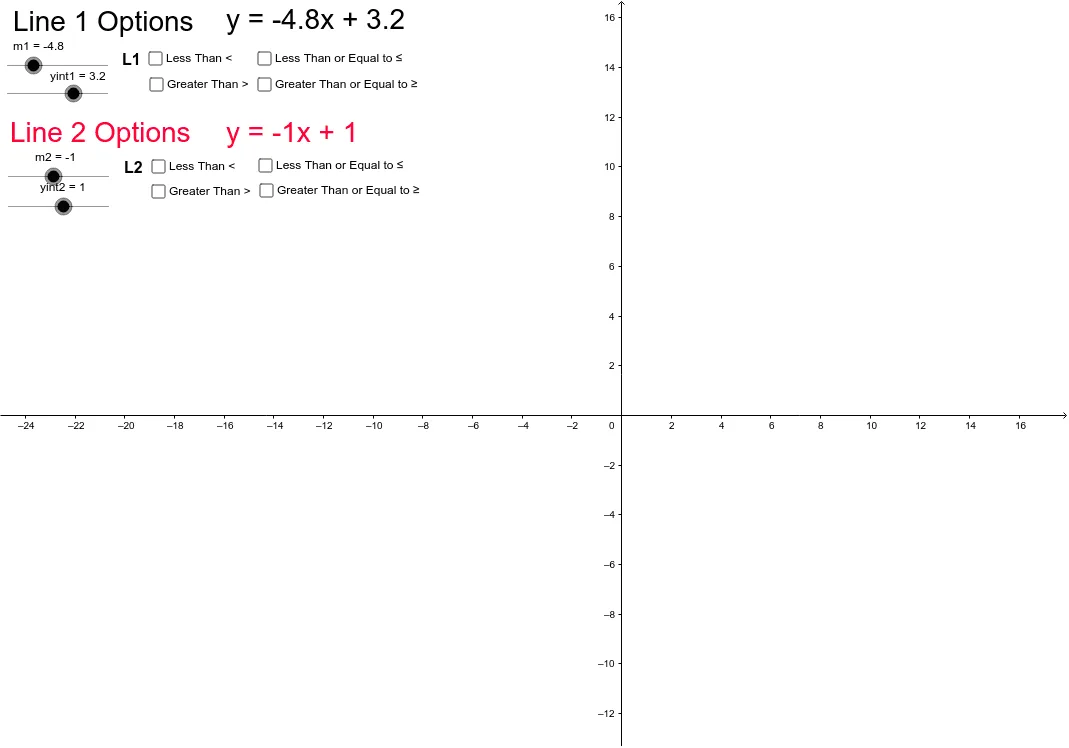
This example dynamically demonstrates the solution set of linear inequalities on a coordinate plane using sliders. It covers core math concepts like linear inequalities, solution sets, number line representations, and region partitioning. GeoGebra commands and objects such as m1, yint1, a, a_1, a_2, a_3, b, c, d, e, text1, text2, m2, yint2, f, f_1, f_2, f_3, h, i, j, g, text3, text4, text5, text6 are used to draw lines, label inequality solutions, and adjust parameters dynamically. Suitable for high school students learning the geometric meaning of linear inequalities and classroom demonstrations.