
Linear Equations & Optimization Demo
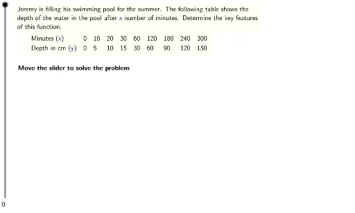
Loading the math board and drawing, please wait…
This example demonstrates the graphical solution of linear equations and optimization problems using GeoGebra. Core math concepts include linear equations, logarithmic functions, linear programming, probability & statistics, and linear regression. Construction highlights from the summary involve commands like LaTeX, Corner, If, Zip, Append, TableText, and objects such as timeDepthratio, depthratio, stepMax, stepper, steps, etc., making it suitable for high school and above for understanding complex mathematical model construction and visualization.
GeoGebra Commands & Parameters
LaTeX(steps) → counterLaTeX("\text{Move the slider to solve the problem}") → text0LaTeX("\text{Use the buttons below to return to the original problem or}\cr\text{randomly generate a similar practice problem.}") → RandomizationTextCorner(1) → ACorner(3) → BIf(direction ≟ 0, "filling", "emptying") → directionWordLaTeX((("\text{Jeremy is " * directionWord) * " his swimming pool for the summer. The following table shows the}\cr\text{depth of the water in the pool after }\textcolor{#000099}{x}\text{ number of minutes. Determine the key features}\cr\text{of this function.}")) → ProblemZip((timeratio * k), k, intervalScales) → TimeIntervalsAppend(0, Sequence[Sum[TimeIntervals, k], k, 1, 8]) → TimesZip((depthratio * k), k, intervalScales) → DepthIntervalsAppend(0, Sequence[Sum[DepthIntervals, k], k, 1, 8]) → DepthValuesIf(direction ≟ 0, DepthValues, Append[DepthValues(9), Sequence[DepthValues(9) - Sum[DepthIntervals, k], k, 1, 8, 1]]) → DepthsLaTeX("\text{Determine whether the function is linear.}") → text1LaTeX("\text{Identify the intercepts of the function based on the information in the table.}") → text3TableText({Append[LaTeX["\text{Minutes (}\textcolor{#000099}{x}\text{)}"], Times], Append[LaTeX["\text{Depth in cm (}\textcolor{#000099}{y}\text{)}"], Depths]}) → ProblemDataLaTeX((((((((("\text{The function intersects the }\textcolor{#000099}{y}\text{-axis at the point }\textcolor{#000099}{" * Yintercept) * "}\text{ as indicated in the table,}\cr\text{and it also intersects the }\textcolor{#000099}{x}\text{-axis at }\textcolor{#000099}{") * Xintercept) * "}\text{.}\cr\text{}\cr\text{Therefore, the }\textcolor{#000099}{y}\text{-intercept is }\textcolor{#000099}{") * Yintercept) * "}\text{ and the }\textcolor{#000099}{x}\text{-intercept is }\textcolor{#000099}{") * Xintercept) * "}\text{.}")) → text4LaTeX("\text{Determine whether the function is increasing or decreasing.}") → text5If(direction ≟ 0, "increasing", "decreasing") → functionWordIf(direction ≟ 0, "increase", "decrease") → yWordLaTeX((((("\text{As the }\textcolor{#000099}{x}\text{-values increase, the }\textcolor{#000099}{y}\text{-values " * yWord) * ". Therefore, the function is}\cr\text{") * functionWord) * ".}")) → text6LaTeX("\text{Determine where the function is positive and negative.}") → text7If(direction ≟ 0, ">", "<") → relationSignIf(direction ≟ 0, 0, Times(9)) → keyXIf(direction ≟ 0, "greater", "less than") → relationWordLaTeX("\text{Determine the relative minimum and maximum of the function.}") → text9If(direction ≟ 0, LaTeX["\text{whatever time Jeremy stops filling the pool, or}\cr\text{when the pool starts overflowing. The problem did not specify when this would be.}"], LaTeX[(("\textcolor{#000099}{" * Yintercept) * "}\text{ before the pool begins to empty.}")]) → relMaxIf(direction ≟ 0, (0, 0), (Times(9), 0)) → relMinLaTeX((("\text{The relative maximum occurs at " * relMax) * "}")) → text10bLaTeX("\text{Identify the domain of the function.}") → text11LaTeX((("\text{We can see from the table that the differences for }\textcolor{#000099}{y}\text{ are always }\textcolor{#000099}{\frac{1}{" * timeDepthratio) * "}}\text{ the}\cr\text{differences in }\textcolor{#000099}{x}\text{, indicating that the rate of change is constant. Therefore, the}\cr\text{scenario described here is linear.}")) → text2LaTeX((((((((("\text{The }\textcolor{#000099}{y}\text{-values are positive for all }\textcolor{#000099}{x}\text{-values " * relationWord) * " than }\textcolor{#000099}{") * keyX) * "}\text{. Therefore, the}\cr\text{function is positive when }\textcolor{#000099}{x ") * relationSign) * " ") * keyX) * "}\text{.}\cr\text{}\cr\text{The }\textcolor{#000099}{y}\text{-values are never negative in this scenario. Therefore, the function is never}\cr\text{negative. }")) → text8LaTeX((("\text{The relative minimum occurs at }\textcolor{#000099}{" * relMin) * "}\text{, because there cannot be a negative}\cr\text{amount of water in the pool.}")) → text10LaTeX((((("\text{The least }\textcolor{#000099}{x}\text{-value is }\textcolor{#000099}{0}\text{, the time when Jeremy starts " * directionWord) * " the pool. The}\cr\text{greatest }\textcolor{#000099}{x}\text{-value is whatever time Jeremy stops ") * directionWord) * " the pool. Additionally, }\cr\textcolor{#000099}{x}\text{ can be any real number because time is continuous.}")) → text12