
Interactive Linear Regression with MSE function
Loading the math board and drawing, please wait…
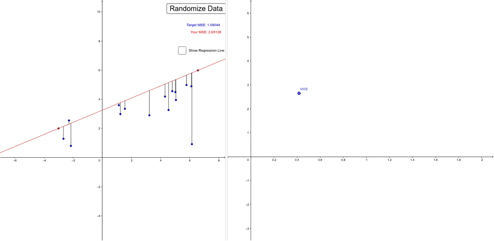
This interactive GeoGebra example demonstrates how to fit an optimal linear regression line by minimizing the Mean Squared Error (MSE) function. Core mathematical concepts include linear regression, least squares method, MSE loss function, residuals, and statistical characteristics like the mean of data points. Constructed using key GeoGebra commands such as Line, mean, Sum, OrthogonalLine, Intersect, Segment, and Residual, along with interactive objects like button1 and various point pairs, the applet dynamically visualizes the perpendicular residuals and the summation of squared errors. It is highly suitable for teaching and learning regression analysis, statistical modeling, and optimization in high school or university-level data science and calculus courses.
GeoGebra Commands & Parameters
Line(A, B) → amean(A2:A16) → A18mean(B2:B16) → B18Sum(F2:F16) → F18Sum(G2:G16) → G18Line(D, C) → bOrthogonalLine(O11, xAxis) → cIntersect(b, c) → ESegment(E, O11) → dResidual(O1, b) → eResidual(O2, b) → fResidual(O10, b) → gResidual(O3, b) → hResidual(O12, b) → iResidual(O4, b) → jResidual(O13, b) → kResidual(O5, b) → lResidual(O14, b) → mResidual(O6, b) → nResidual(O8, b) → pResidual(O15, b) → qResidual(O9, b) → rResidual(O7, b) → sResidual(O10, a) → tResidual(O11, a) → a_1Residual(O1, a) → b_1Residual(O2, a) → c_1Residual(O12, a) → d_1Residual(O3, a) → e_1Residual(O13, a) → f_1Residual(O4, a) → g_1Residual(O14, a) → h_1Residual(O5, a) → i_1Residual(O6, a) → j_1Residual(O15, a) → k_1Residual(O7, a) → m_1Residual(O8, a) → n_1Residual(O9, a) → p_1Sum(I2:I16) → I18Sum(J2:J16) → J18
AI Drawing Prompt Reference
Draw an interactive linear regression graph that demonstrates how to fit a line by minimizing the mean squared error (MSE) function. The graph should include a linear regression line, a mean point, a vertical line, an intersection point, a segment, residuals, a button, and multiple point pairs. The construction order is: first draw the regression line, then calculate the mean and sum of squared errors for the data points, next find the projection point via a vertical line, then draw residual segments and the vertical projection line, and finally add the interactive button and point pairs for dynamic adjustment and visualization of errors.
The prompt above was compiled from the original drawing commands and is for reference only.