
Interactive Linear Regression
Loading the math board and drawing, please wait…
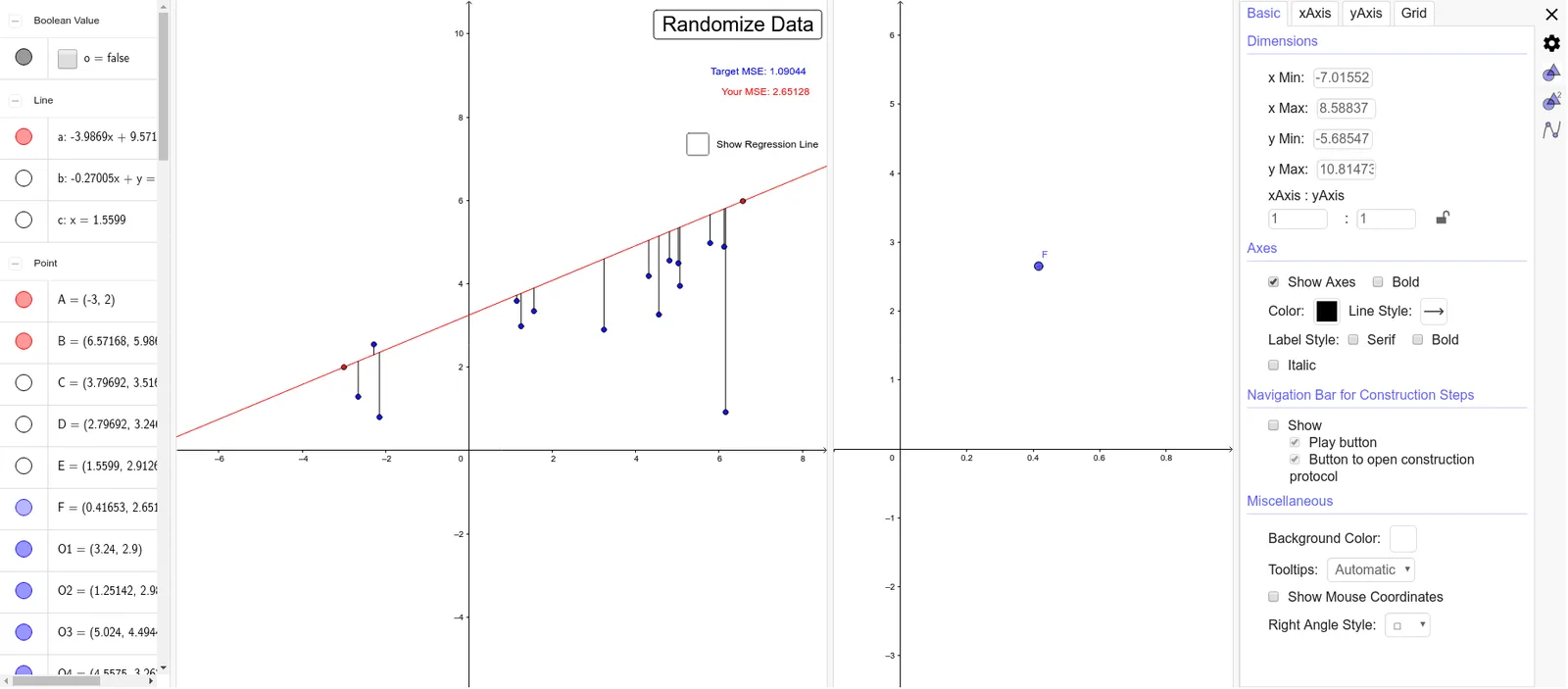
This interactive linear regression example allows users to visualize how a best‑fit line is constructed from a set of data points. It demonstrates key concepts such as linear regression, arithmetic operations (mean, sum), vector geometry in the plane, coordinate geometry (orthogonal lines and intersections), and residual analysis. The GeoGebra construction uses commands like Line, mean, Sum, OrthogonalLine, Intersect, Segment, and Residual, together with numerous objects (buttons, points, lines) to enable dynamic fitting. It is suitable for high‑school and university students studying statistics, data analysis, and mathematical modeling.
GeoGebra Commands & Parameters
Line(A, B) → amean(A2:A16) → A18mean(B2:B16) → B18Sum(F2:F16) → F18Sum(G2:G16) → G18Line(D, C) → bOrthogonalLine(O11, xAxis) → cIntersect(b, c) → ESegment(E, O11) → dResidual(O1, b) → eResidual(O2, b) → fResidual(O10, b) → gResidual(O3, b) → hResidual(O12, b) → iResidual(O4, b) → jResidual(O13, b) → kResidual(O5, b) → lResidual(O14, b) → mResidual(O6, b) → nResidual(O8, b) → pResidual(O15, b) → qResidual(O9, b) → rResidual(O7, b) → sResidual(O10, a) → tResidual(O11, a) → a_1Residual(O1, a) → b_1Residual(O2, a) → c_1Residual(O12, a) → d_1Residual(O3, a) → e_1Residual(O13, a) → f_1Residual(O4, a) → g_1Residual(O14, a) → h_1Residual(O5, a) → i_1Residual(O6, a) → j_1Residual(O15, a) → k_1Residual(O7, a) → m_1Residual(O8, a) → n_1Residual(O9, a) → p_1Sum(I2:I16) → I18Sum(J2:J16) → J18