
Linear Correlation Coefficients Comparison
Loading the math board and drawing, please wait…
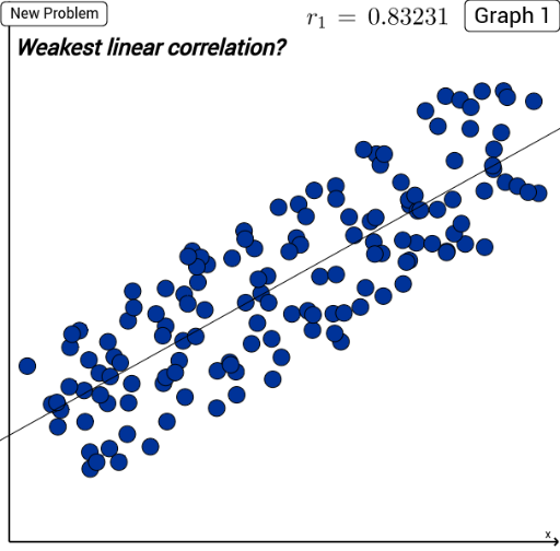
① This example demonstrates a side‑by‑side comparison of the linear correlation coefficients of two random scatterplots, visualizing differences in correlation strength. ② Core mathematical concepts include linear correlation, Pearson product‑moment correlation coefficient (PMCC), linear regression fitting, and scatter‑plot distribution characteristics. ③ Construction highlights: Sequence generates random point sets; If handles conditional logic; PMCC computes correlation coefficients; FitLineY fits regression lines; LaTeX renders formulas; AxisStepX sets axis steps. Key objects: l_0, type_1, xrnd_1, elem_1, l_n, l_p, corner1, corner3, strength_1, L_1, pts_1, r_1, and their counterparts for the second dataset. ④ Suitable for high‑school statistics and probability courses, introductory university statistics, and data‑analysis workshops.
GeoGebra Commands & Parameters
Sequence((2 * random()) - 1 + i, i, 1.5, 15.9, 0.1) → xrnd_1If(type_1 ≟ 0, Element[l_0, elem_1], If[type_1 < 0, Element[l_n, elem_1], Element[l_p, elem_1]]) → L_1Sequence((Element[xrnd_1, j], ((((elem_1 + 2) * 2) * random()) - (elem_1 + 2)) / strength_1 + L_1(Element[xrnd_1, j])), j, 1, Length[xrnd_1]) → pts_1PMCC(pts_1) → r_1FitLineY(pts_1) → reg_1Sequence((2 * random()) - 1 + i, i, 1.5, 15.9, 0.1) → xrnd_2If(type_2 ≟ 0, Element[l_0, elem_2], If[type_2 < 0, Element[l_n, elem_2], Element[l_p, elem_2]]) → L_2Sequence((Element[xrnd_2, j], ((((elem_2 + 2) * 2) * random()) - (elem_2 + 2)) / strength_2 + L_2(Element[xrnd_2, j])), j, 1, Length[xrnd_2]) → pts_2FitLineY(pts_2) → reg_2PMCC(pts_2) → r_2LaTeX(r_1, true, true) → txtr1LaTeX(r_2, true, true) → txtr2AxisStepX() → xx
AI Drawing Prompt Reference
Create a statistical chart for side-by-side comparison of the linear correlation coefficients of two random scatterplots, visualizing differences in correlation strength. The chart includes two scatterplots, each with a set of randomly generated points and a fitted regression line. Display the Pearson correlation coefficient for each scatterplot using LaTeX formulas, and set axis steps for clarity. The construction sequence: first generate random point sets, then compute correlation coefficients and regression lines, and finally render the formulas.
The prompt above was compiled from the original drawing commands and is for reference only.