
Linear Regression vs. Best Fit Line
Loading the math board and drawing, please wait…
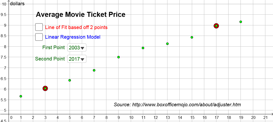
This example demonstrates the difference between linear regression and the best fit line. It involves key mathematical concepts such as linear regression and residual sum of squares. Using GeoGebra commands like Sequence, FitLineY, and ResidualPlot, it constructs a clear and intuitive graph. Suitable for high school mathematics education and learning.
GeoGebra Commands & Parameters
Sequence((Element[yr2000, i], Element[price, i]), i, 1, Length[yr2000]) → observedFitLineY(fit_{2PT}) → lin_{2PT}FitLineY(observed) → lin_{REG}Corner(1) → G1Corner(3) → G4ResidualPlot(observed, lin_{REG}) → resid_{REG}Sequence((yr2000(n), lin_{REG}(yr2000(n))), n, 1, Length[yr2000]) → pred_{REG}ResidualPlot(observed, lin_{2PT}) → resid_{2PT}SumSquaredErrors(observed, lin_{REG}) → sumsquared_{REG}SumSquaredErrors(observed, lin_{2PT}) → sumsquared_{2PT}Sum((y(resid_{2PT}))^(2)) → manualsumsq_{2PT}Sum((y(resid_{REG}))^(2)) → mansumsq_{REG}Sequence((yr2000(n), lin_{2PT}(yr2000(n))), n, 1, Length[yr2000]) → pred_{2PT}PMCC(yr2000, price) → r
AI Drawing Prompt Reference
Draw a graph showing the difference between linear regression and the best fit line, including two sets of data points and their fitting lines, with residual plots and predicted values marked, then calculate and compare the residual sum of squares and manually computed squares for both datasets, distinguishing them with different colors, and display the correlation coefficient.
The prompt above was compiled from the original drawing commands and is for reference only.