
Length vs. Temperature - Square Root Simulation
Loading the math board and drawing, please wait…
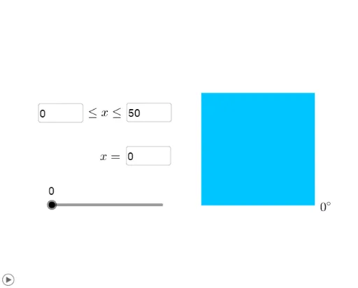
This example demonstrates the simulation of the relationship between length and temperature using a square root function. It involves core mathematical concepts such as square root functions, geometric constructions, and data simulation. Key GeoGebra commands like Polygon, Textfield, Segment, If, Point, and Mirror are used to create dynamic visualizations, with sliders to simulate temperature changes and observe length variations. Suitable for high school mathematics education, focusing on function graphs, geometric transformations, and data visualization.
GeoGebra Commands & Parameters
Polygon(A, B, 4) → poly1, f, g, h, i, C, DTextfield(cmin) → InputBox1Textfield(cmax) → InputBox2Textfield(a) → InputBox3Textfield(outputmin) → InputBox4Textfield(outputmax) → InputBox5Segment(E, F) → jTextfield(a) → InputBox3_1Textfield(outputmin) → InputBox4_1Textfield(outputmax) → InputBox5_1Segment(E_1, F_1) → j_1Polygon(A_1, B_1, 4) → poly1_1, f_1, g_1, h_1, i_1, C_1, D_1If(ZeroToOne < 37 / 256, 0, 37 / 256 ≤ ZeroToOne ≤ 179 / 256, (48.845 * (ZeroTo256 - 37)^(1 / 3) / 256), ZeroToOne > 179 / 256, 1) → redIf(ZeroToOne < 94 / 256, 255, 94 / 256 ≤ ZeroToOne ≤ 210 / 256, ((-2.198 * (ZeroTo256 - 210))) / 256, ZeroToOne > 210 / 256, 0) → blueTextfield(lengthmin) → InputBox6Textfield(lengthmax) → InputBox7Point(Circle[G, abs(n(a))]) → HSegment(G, H) → kTextfield(n) → InputBox8Mirror(H, G) → H'Segment(G, H') → lPoint(Circle[I, abs(puzzle(a))]) → JSegment(I, J) → mMirror(J, I) → J'Segment(I, J') → r