
Leaves in Nature (Surface Example)
Loading the math board and drawing, please wait…
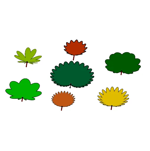
This example demonstrates the surface morphology of leaves in nature. It involves core concepts of trigonometry and coordinate geometry. Using commands like CurveCartesian and Surface in GeoGebra, a 3D model of a leaf can be constructed. Suitable for high school and above students or teachers for teaching and learning.
GeoGebra Commands & Parameters
Textfield(r) → ChampTexte1CurveCartesian(x(C) + (((sin(i) + sin((25 * i)) / 12) * R) * cos(i)), y(C) + (((sin(i) + sin((25 * i)) / 12) * R) * sin(i)), i, 0, 6.283185307179586) → cCurveCartesian(x(B) + (((sin(i) + sin((16 * i)) / 3) * R) * cos(i)), y(B) + (((sin(i) + sin((16 * i)) / 3) * R) * sin(i)), i, 0, 6.283185307179586) → bCurveCartesian(x(D) + (((sin(i) + sin((45 * i)) / 12) * R) * cos(i)), y(D) + (((sin(i) + sin((45 * i)) / 12) * R) * sin(i)), i, 0, 6.283185307179586) → dCurveCartesian(x(A) + ((r(i) * R) * cos(i)), y(A) + ((r(i) * R) * sin(i)), i, 0, t) → hSegment(E, H) → iSegment(C, M) → kSegment(G, I) → lSegment(F, J) → mSegment(B, K) → nSegment(D, L) → pCurveCartesian(x(F) + (((sin(i) + sin((55 * i / 15))) * R / 1.5) * cos(i)), y(F) + (((sin(i) + sin((55 * i / 15))) * R / 1.5) * sin(i)), i, 0, 18.84956) → fCurveCartesian(x(G) + (((sin(i) + sin((75 * i / 20))) * R / 1.5) * cos(i)), y(G) + (((sin(i) + sin((75 * i / 20))) * R / 1.5) * sin(i)), i, 0, 15.707963267948966) → gCurveCartesian(x(E) + (((sin(i) + sin((25 * i / 4))) * R / 2) * cos(i)), y(E) + (((sin(i) + sin((25 * i / 4))) * R / 2) * sin(i)), z(E), i, 0, 6.28319) → eCurveCartesian(x(E) + (0.1 * cos(i)), y(E) + (0.1 * sin(i)), z(E), i, 0, (2 * π)) → oSurface((b * e(a)) + ((1 - b) * o(a)), a, 0, (2 * π), b, 0, 1) → qCurveCartesian(x(C) + (0.1 * cos(i)), y(C) + (0.1 * sin(i)), z(C), i, 0, (2 * π)) → sSurface((b * c(a)) + ((1 - b) * s(a)), a, 0, (2 * π), b, 0, 1) → uCurveCartesian(x(G) + (0.1 * cos(i)), y(G) + (0.1 * sin(i)), z(G), i, 0, (2 * π)) → vSurface((b * g(a)) + ((1 - b) * v(a)), a, 0, (5 * π), b, 0, 1) → wCurveCartesian(x(F) + (0.1 * cos(i)), y(F) + (0.1 * sin(i)), z(F), i, 0, (2 * π)) → a_1Surface((b * f(a)) + ((1 - b) * a_1(a)), a, 0, (5 * π), b, 0, 1) → b_1CurveCartesian(x(D) + (0.1 * cos(i)), y(D) + (0.1 * sin(i)), z(D), i, 0, (2 * π)) → c_1Surface((b * d(a)) + ((1 - b) * c_1(a)), a, 0, (5 * π), b, 0, 1) → d_1CurveCartesian(x(B) + (0.1 * cos(i)), y(B) + (0.1 * sin(i)), z(B), i, 0, (2 * π)) → e_1Surface((b * b(a)) + ((1 - b) * e_1(a)), a, 0, (5 * π), b, 0, 1) → f_1CurveCartesian(x(A) + (0.1 * cos(i)), y(A) + (0.1 * sin(i)), z(A), i, 0, (2 * π)) → g_1CurveCartesian(x(A) + ((r(i) * R / 1.25) * cos(i)), y(A) + ((r(i) * R / 1.25) * sin(i)), i, 0, t) → aSurface((b * a(a)) + ((1 - b) * g_1(a)), a, 0, (5 * π), b, 0, 1) → h_1Segment(A, N) → i_1
AI Drawing Prompt Reference
Draw the surface morphology of leaves in nature to showcase their 3D structure. Use sinusoidal functions and parametric equations to generate the outlines of the leaves, combining curves with different parameters to form the立体 effect of the leaves. Start by drawing the basic outlines, add detailed curves, and finally combine the curves with planes to generate 3D surfaces, presenting a realistic leaf shape.
The prompt above was compiled from the original drawing commands and is for reference only.