
Lagrange Multipliers for Conditional Extrema
Loading the math board and drawing, please wait…
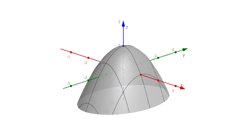
This example demonstrates the solution of conditional extrema using the Lagrange multiplier method. It visually illustrates the principle of the multiplier method through the graphical representation of the objective function and constraint. Key mathematical concepts include conditional extrema, Lagrange multipliers, gradient vectors, and the geometric meaning of functions. Construction highlights the use of GeoGebra commands and objects such as Derivative (derivative), Point (point), Vector (vector), SelectedElement (selected element), CurveCartesian (Cartesian curve), Segment (segment), Tangent (tangent), and others like g3, g2, ell3, ell2, ell1, g1, listg, zyl_1, f, w_1, w_2, w_3, w_5, f_x, P_1, f_y, g_x, g_y, gradf_{P1}, Text1, w_4, g, b, P_2, P_3, gradf_{P2}, gradg_{P2}, gradg_{P3}, gradf_{P3}, zyl_2, zyl_3, gradg_{P1}, Text3, k21, k22, S_1, s_1, S_2, S_3, s_2. Suitable for high school and above students learning optimization problems.
GeoGebra Commands & Parameters
Derivative(f, x) → f_xPoint(ell1) → P_1Derivative(f, y) → f_yDerivative(g1, x) → g_xDerivative(g1, y) → g_yVector((f_x(x(P_1), y(P_1)), f_y(x(P_1), y(P_1)))) → gradf_{P1}SelectedElement(listg) → gSelectedIndex(listg) → bPoint(ell2) → P_2Point(ell3) → P_3Vector((f_x(x(P_2), y(P_2)), f_y(x(P_2), y(P_2)))) → gradf_{P2}Vector((g_x(x(P_2), y(P_2)), g_y(x(P_2), y(P_2)))) → gradg_{P2}Vector((g_x(x(P_3), y(P_3)), g_y(x(P_3), y(P_3)))) → gradg_{P3}Vector((f_x(x(P_3), y(P_3)), f_y(x(P_3), y(P_3)))) → gradf_{P3}Vector((g_x(x(P_1), y(P_1)), g_y(x(P_1), y(P_1)))) → gradg_{P1}CurveCartesian(t, sqrt(1 - t^(2) / 2), 1 / 2 - (3 / 4 * t^(2)), t, -2, 2) → k21CurveCartesian(t, (-sqrt(1 - t^(2) / 2)), 1 / 2 - (3 / 4 * t^(2)), t, -20, 2) → k22Segment(P_1, S_1) → s_1Segment(P_2, S_2) → s_2Segment(P_3, S_3) → s_3CurveCartesian(cos(t), sin(t), f(cos(t), sin(t)), t, 0, (2 * pi)) → k1CurveCartesian((sqrt(2) * cos(t)), sin(t), f((sqrt(2) * cos(t)), sin(t)), t, 0, (2 * pi)) → k2CurveCartesian(cos(t), (sqrt(2) * sin(t)), f(cos(t), (sqrt(2) * sin(t))), t, 0, (2 * pi)) → k3Tangent(S_1, k1) → t_1Segment(S_1 - UnitVector[t_1], S_1 + UnitVector[t_1]) → t11Tangent(S_2, k2) → t_2Segment(S_2 - UnitVector[t_2], S_2 + UnitVector[t_2]) → t21Tangent(S_3, k3) → t_3Segment(S_3 - UnitVector[t_3], S_3 + UnitVector[t_3]) → t31