Investigating the Properties of an Isosceles Trapezoid

GeoGebra Commands & Parameters

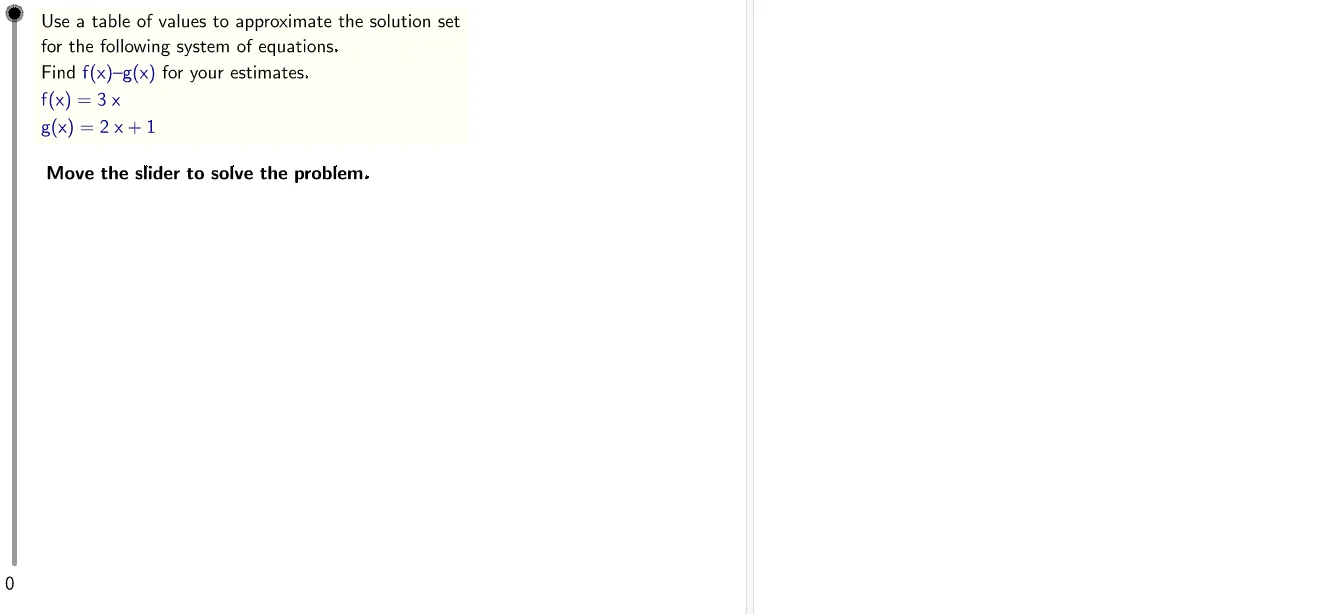
1. LaTeX(steps) → counter
2. LaTeX("\text{Move the slider to solve the problem.}") → text0
3. LaTeX("\text{Use the buttons below to return to the original}\cr\text{problem or randomly generate a similar practice}\cr\text{problem.}") → RandomizationText
4. Corner(2, 3) → topright
5. Corner(2, 1) → bottomleft
6. Simplify((ga * x) + gb) → g
7. If(gb > 0, LaTeX[("+" * gb)], LaTeX[gb]) → gadd
8. If(ydiff ≟ 0, LaTeX["satisfies"], LaTeX["approximately satisfies"]) → sat
9. If(ydiff ≟ 0, LaTeX["x-coordinate"], LaTeX["approximate x-coordinate"]) → coord
10. If(ydiff ≟ 0, LaTeX["solution"], LaTeX["approximate solution"]) → soln
11. LaTeX((((("\text{Use a table of values to approximate the solution set}\cr\text{for the following system of equations.}\cr\text{Find }\textcolor{#000099}{f(x) – g(x)}\text{ for your estimates.}\cr\textcolor{#000099}{f(x)=" * f) * "}\cr\textcolor{#000099}{g(x)=") * g) * "}")) → Problem
12. LaTeX((((("\text{Create a table of values for }\textcolor{#000099}{f(x) = " * f) * "}\text{ and }\cr\textcolor{#000099}{g(x) = ") * g) * "}\text{.}")) → text1
13. Sequence(i, i, (-xscale), xscale) → xvalues
14. Zip(f(j), j, xvalues) → fvalues
15. Zip(g(j), j, xvalues) → gvalues
16. Zip(j - k, j, fvalues, k, gvalues) → fgdiffs
17. TableText({Append[LaTeX["\textcolor{#000099}{x}"], xvalues], Append[LaTeX["\textcolor{#000099}{f(x)}"], fvalues], Append[LaTeX["\textcolor{#000099}{g(x)}"], gvalues], Append[LaTeX["\textcolor{#000099}{f(x)-g(x)}"], fgdiffs]}, "vr") → text2
18. LaTeX("\text{In column }\textcolor{#000099}{f(x) – g(x)}\text{, look for sign changes.}") → text3
19. Sequence(If[sgn(fgdiffs(k)) ≟ sgn(fgdiffs(k + 1)), "F", "T"], k, 1, Length[fgdiffs] - 2) → signChange
20. Length(signChange \ {"F"}) → numrows
21. IndexOf("T", signChange) → firstchange
22. LaTeX((((("\text{There is a sign change from }\textcolor{#000099}{x=" * xvalues(firstchange)) * "}\text{ to }\textcolor{#000099}{x=") * xvalues(firstchange + numrows)) * "}\text{.}")) → text4
23. Sequence(fgdiffs(k), k, firstchange, firstchange + numrows) → fgdiffsS
24. Sequence(fvalues(k), k, firstchange, firstchange + numrows) → fvaluesS
25. Sequence(gvalues(k), k, firstchange, firstchange + numrows) → gvaluesS
26. Sequence(xvalues(k), k, firstchange, firstchange + numrows) → xvaluesS
27. TableText({Append[LaTeX["\textcolor{#000099}{x}"], xvaluesS], Append[LaTeX["\textcolor{#000099}{f(x)}"], fvaluesS], Append[LaTeX["\textcolor{#000099}{g(x)}"], gvaluesS], Append[LaTeX["\textcolor{#000099}{f(x)-g(x)}"], fgdiffsS]}, "vr") → text4b
28. If(solx ≟ floor(solx), "int", "rat") → version
29. LaTeX(LaTeX["\text{The sign change occurs between adjacent integers}\cr\text{so look at values in between them.}"]) → text5B
30. Sequence(k, k, xvalues(firstchange), xvalues(firstchange) + 1, 0.1) → xvalues2
31. Zip(f(k), k, xvalues2) → fvalues2
32. Zip(g(k), k, xvalues2) → gvalues2
33. Zip(j - k, j, fvalues2, k, gvalues2) → fgdiffs2
34. Sequence(If[sgn(fgdiffs2(k)) ≟ sgn(fgdiffs2(k + 1)), "F", "T"], k, 1, Length[fgdiffs2] - 2) → signChange2
35. LaTeX((((((("\text{Between these points, at }\textcolor{#000099}{x=" * solx) * "}\text{,}\cr\textcolor{#000099}{f(x)-g(x)=") * yapproxf) * "- (") * yapproxg) * ")= 0}\text{.}")) → text5
36. LaTeX((((((((("\text{This tells us the curves }\textcolor{#000099}{f}\text{ and }\textcolor{#000099}{g}\text{ intersect at }\cr\textcolor{#000099}{x = " * xapprox) * "}\text{. The corresponding y-value is}\cr\text{}\textcolor{#000099}{") * yapproxf) * "}\text{. }\text{Therefore, the solution set of this}\cr\text{system is }\textcolor{#000099}{(") * xapprox) * ", ") * yapproxf) * ")}\text{.}")) → text6
37. TableText({Append[LaTeX["\textcolor{#000099}{x}"], xvalues2], Append[LaTeX["\textcolor{#000099}{f(x)}"], fvalues2], Append[LaTeX["\textcolor{#000099}{g(x)}"], gvalues2], Append[LaTeX["\textcolor{#000099}{f(x)-g(x)}"], fgdiffs2]}, "vr") → text5C
38. LaTeX((((((((("\text{This tells us the curves }\textcolor{#000099}{f}\text{ and }\textcolor{#000099}{g}\text{ intersect at }\cr\text{approximately }\textcolor{#000099}{x \approx " * solx) * "}\text{. The corresponding y-value}\cr\text{is approximately }\textcolor{#000099}{") * soly) * "}\text{. }\text{Therefore, the approximate}\cr\text{solution set of this system is }\textcolor{#000099}{(") * solx) * ", ") * soly) * ")}\text{.}")) → text6B
39. Length(signChange2 \ {"F"}) → Sign2Count
40. LaTeX("\text{Since zero once again doesn't show up in the }\cr\textcolor{#000099}{f(x)-g(x)}\text{ values, the actual intersection falls}\cr\text{between table values. The solution above rounds}\cr\text{to the nearest tenth.}") → text6C