Investigating the Domain and Range of Linear Functions

Loading the math board and drawing, please wait…

2015-12-31 07:06

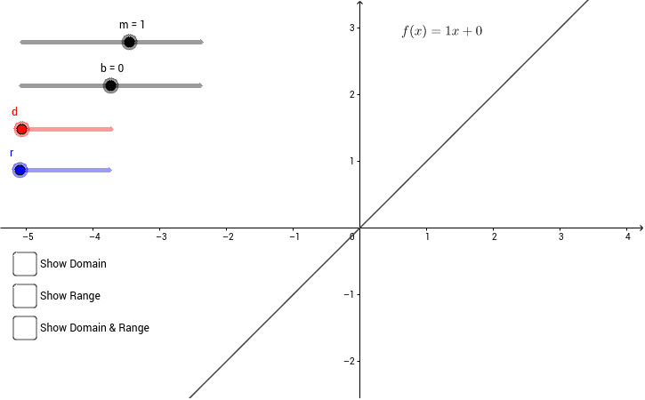
This applet visualizes the domain and range of a linear function f(x)=mx+b. Users can adjust the slope m and y-intercept b to observe changes in the function's graph. Key mathematical concepts include linear functions, domain, and range. GeoGebra commands used include Segment and If. Suitable for high school mathematics education and learning.

GeoGebra Commands & Parameters

Segment((-6, 0), (d, 0)) → domain
If(a, Segment[(0, f(-6)), (0, f(d))], Segment[(0, f(-6)), (0, f(r))]) → range
If(a ∨ c, Point[{d, 0}]) → dtracer
If(a ∨ c, (d, f(d))) → fxdtracer
If(a, Point[{d, f(d)}], If[e, Point[{r, f(r)}]]) → fxrtracer
If(a, Point[{0, f(d)}], If[e, Point[{0, f(r)}]]) → rtracer
If(a ∨ c, Segment[(d, 0), (d, f(d))]) → g
If(e, Segment[(0, r), (r, f(r))], If[a, Segment[(0, d), (d, f(d))]]) → h

AI Drawing Prompt Reference

Draw a linear function f(x)=mx+b graph where m and b can be adjusted with sliders. Draw a line segment on the x-axis to represent the domain. Then, plot the intersection points of the function graph with the y-axis and x-axis. Finally, draw a line segment from the y-axis to the function graph to represent the range.

The prompt above was compiled from the original drawing commands and is for reference only.