
Introduction to Sketching Curves with Polar Equations
Loading the math board and drawing, please wait…
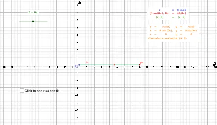
This example introduces sketching curves using polar equations, providing an interactive geometric construction that helps students visualize shapes in the polar coordinate system. The core mathematical concepts include polar representation, angle measurement, rotation transformations, and curve loci. The construction utilizes GeoGebra commands such as Rotate, Angle, Segment, FractionText, AngularBisector, Point, and Midpoint to guide learners in linking polar equations to their Cartesian graphs. It is suitable for high school or early university mathematics courses covering analytic geometry, functions, or pre‑calculus.
GeoGebra Commands & Parameters
Rotate(A, a, B) → P'Angle(A, B, P') → αSegment(B, P) → fFractionText(b) → text1AngularBisector(A, B, P') → gPoint(g) → DPoint(f) → OSegment(O, P') → hMidpoint(O, P) → CRotate(A, (-(180°)), O) → A'Angle(A', O, A) → β
AI Drawing Prompt Reference
Draw a curve described by a polar equation. The drawing should include a center point, a rotated point, an angle measurement point, a segmented line, and a midpoint. The construction order is: first determine the center point, then rotate a point, measure the angle, draw the segmented line, and find the midpoint. Ensure the curve shape is clearly shown in the polar coordinate system.
The prompt above was compiled from the original drawing commands and is for reference only.