Introduction to Simple Linear Regression: Visualizing Error Sum of Squares

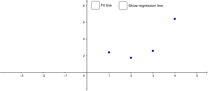
① This example demonstrates simple linear regression using four scatter points and an adjustable fitted line, showing how changing the slope and intercept affects the sum of squared errors. ② Core mathematical concepts include linear regression, least squares method, residuals (errors), and correlation coefficient, providing a foundation for statistical data fitting. ③ Construction details: GeoGebra commands Segment and FitLineY are used; objects include points A, B, C, D, line m, sliders for intercept (c) and slope (m), error segments e_1 to e_4, and displayed values for sum of squares (SS), correlation coefficient (r), and regression equation text. ④ Suitable for high school or introductory college statistics students, this interactive tool helps learners grasp the geometric meaning of regression lines and the least squares principle, and serves as an effective classroom demonstration for exploring how parameter adjustments influence model fit.