Interactive Histograms in GeoGebra

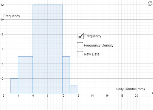
This GeoGebra example demonstrates the construction and interpretation of histograms, showing how data distribution can be visualized through grouped frequency intervals. Core mathematical concepts include frequency distribution, bin width (class interval), and the relationship between frequency and density in histograms. The construction uses the Histogram command along with objects such as b, a, text1, text2, text3, c, d, e, and text4, likely involving sliders to adjust bin width and dynamic text labels to display counts or frequencies. It may also incorporate optimization problems, similarity transformations, or circle elements to enrich the visualization. Suitable for middle school statistics lessons, high school mathematics, or introductory college statistics courses, this interactive tool helps learners understand data grouping, frequency calculation, and how changing bin width affects the histogram's shape and interpretation.