
Intersection of Cylinder and Cos Surfaces by Roman Chijner
Loading the math board and drawing, please wait…
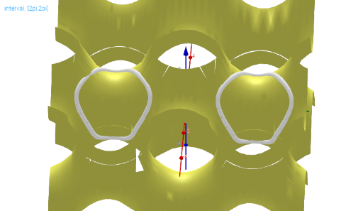
This example demonstrates the intersection of a cylinder and cosine surfaces in the interval [-2π, 2π]. Key mathematical concepts include surface intersection, trigonometric functions, and coordinate geometry. Using GeoGebra commands such as Sequence, Textfield, and InputBox, the dynamic changes in the intersection line are vividly illustrated. Suitable for high school and above students or teachers.
GeoGebra Commands & Parameters
Textfield(x0) → InputBox1Textfield(y0) → InputBox2Sequence(Sequence[CurveCartesian[t, (i * acos((-cos(f1(t))) - cos(t))) + ((j * 2) * π), f1(t), t, (-t_{max}), t_{max}], i, -1, 1, 2], j, -1, 1) → l1Sequence(Sequence[CurveCartesian[x0, (i * acos((-cos(f1(t))) - cos(t))) + ((j * 2) * π), f1(t), t, (-t_{max}), t_{max}], i, -1, 1, 2], j, -1, 1) → l1_{x}Sequence(Sequence[CurveCartesian[t, y0, f1(t), t, (-t_{max}), t_{max}], i, -1, 1, 2], j, -1, 1) → l1_{y}Sequence(Sequence[CurveCartesian[t, (i * acos((-cos(f1(t))) - cos(t))) + ((j * 2) * π), z0, t, (-t_{max}), t_{max}], i, -1, 1, 2], j, -1, 1) → l1_{z}Sequence((i * acos((-cos(x)) - cos(y))), i, -1, 1, 2) → l_fSequence((x - dx)^(2) + (z - dz + ((2 * π) * j))^(2) = r_C^(2), j, -1, 1) → l_CTextfield(z0) → InputBox3Sequence(Sequence[CurveCartesian[t, (i * acos((-cos(f2(t))) - cos(t))) + ((j * 2) * π), f2(t), t, (-t_{max}), t_{max}], i, -1, 1, 2], j, -1, 1) → l2Sequence(Sequence[CurveCartesian[x0, (i * acos((-cos(f2(t))) - cos(t))) + ((j * 2) * π), f2(t), t, (-t_{max}), t_{max}], i, -1, 1, 2], j, -1, 1) → l2_{x}Sequence(Sequence[CurveCartesian[t, y0, f2(t), t, (-t_{max}), t_{max}], i, -1, 1, 2], j, -1, 1) → l2_{y}Sequence(Sequence[CurveCartesian[t, (i * acos((-cos(f2(t))) - cos(t))) + ((j * 2) * π), z0, t, (-t_{max}), t_{max}], i, -1, 1, 2], j, -1, 1) → l2_{z}
AI Drawing Prompt Reference
Visualize the intersection of a cylinder and cosine surfaces within the interval [-2π, 2π], highlighting their 3D spatial relationship. The cylinder is aligned along the x-axis, while the cosine surface rotates around it. Observe how the intersection line changes with parameter adjustments. Project the intersection onto the x-y, x-z, and y-z planes in different colors, and dynamically modify the surface parameters to see the evolution of the intersection shape.
The prompt above was compiled from the original drawing commands and is for reference only.