
Interactive Exploration of Correlation and Linear Fit
Loading the math board and drawing, please wait…
In collections
statistics
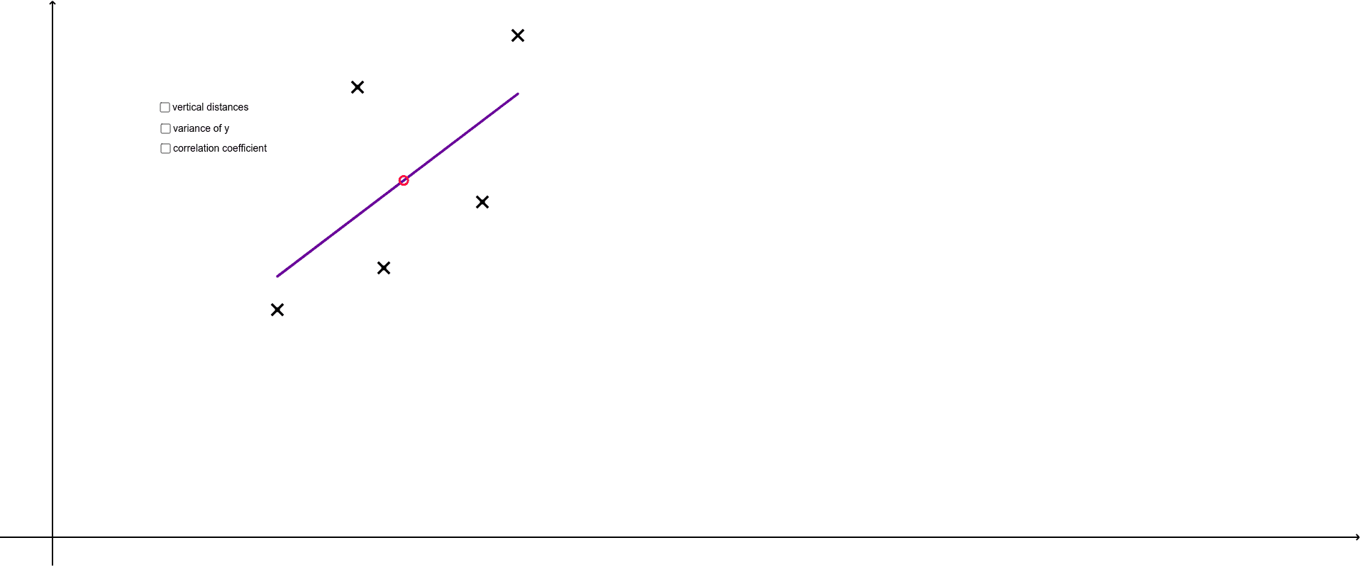
① This example demonstrates the strength and direction of the linear relationship between two variables through a scatter plot and a fitted regression line. ② Core mathematical concepts include Pearson's correlation coefficient (PMCC), covariance (SXY), variances (SXX, SYY), means, standard deviation, and least-squares linear fitting (FitLineY). ③ Construction highlights: FitLineY generates the regression line, PMCC computes the correlation, Variance and Mean calculate statistical measures, Min/Max set data ranges, Intersect and Segment build auxiliary segments, OrthogonalLine draws perpendiculars, Circle adds auxiliary shapes, and lists (list1, list2, list3) manage data points; a dynamic text object (text1) displays statistical results. ④ Suitable for high school or introductory college statistics, this interactive tool helps learners grasp correlation and regression concepts, and serves as a classroom demonstration or self-study resource.
GeoGebra Commands & Parameters
FitLineY(list2) → bPMCC(list2) → cVariance(list1) → aMin(B1:B5) → B7Max(B1:B5) → B8Intersect(b, d) → FIntersect(b, e) → GSegment(F, G) → fSXY(A1:A5) → A9SXX(A1:A5) → A10SXY(list2) → esxySXX(list2) → esxxSYY(list2) → esyyMean(B1:B5) → B6Mean(C1:C5) → C6MeanX(list2) → xbarOrthogonalLine(H, d) → gCircle(H, avesqdist) → hIntersect(h, g, 2) → ISegment(H, I) → iOrthogonalLine(J, d) → jVariance(list1) → varyCircle(J, vary) → kIntersect(k, j, 2) → KSegment(J, K) → lIntersect(a_1, f) → MIntersect(s, f) → NIntersect(r, f) → OIntersect(t, f) → PIntersect(b_1, f) → QIntersect(b_1, c_1) → RIntersect(t, c_1) → SIntersect(r, c_1) → TIntersect(s, c_1) → UIntersect(a_1, c_1) → VSegment(D, V) → d_1Segment(B, U) → e_1Segment(A, T) → f_1Segment(C, S) → g_1Segment(E, R) → h_1Segment(E, Q) → i_1Segment(C, P) → j_1Segment(A, O) → k_1Segment(B, N) → l_1Segment(D, M) → m_1
AI Drawing Prompt Reference
Create a scatter plot of data points with a least-squares regression line showing the linear relationship between two variables. Add an auxiliary line intersecting the regression line, and draw perpendicular segments from the data points to the regression line to illustrate residuals. Also, draw two circles near the data points representing variance and average squared distance, intersecting with perpendicular lines, and connect the intersection points with segments. Finally, include text displaying statistical measures such as correlation coefficient, covariance, variances, means, and the minimum and maximum data values.
The prompt above was compiled from the original drawing commands and is for reference only.