
Interactive Demonstration of Hypothesis Tests for Population Proportion
Loading the math board and drawing, please wait…
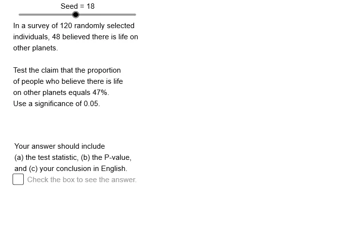
① This GeoGebra example provides an interactive visualization of hypothesis testing for a population proportion p, including setting null and alternative hypotheses, computing test statistics, and displaying rejection regions. ② Core mathematical concepts include hypothesis testing, significance level α, critical values, normal approximation, p-values, standard error, and the normal approximation to the binomial distribution. ③ Construction highlights: commands such as Sequence, Element, Mod, If, Normal, and Min are used to generate random samples and normal distribution curves; sliders (e.g., α, N, P0) control parameters; objects like CnfSq, OpSq series, CV, StdErr0/1 build confidence intervals, test statistics, and decision regions; the interface includes type selection (Type), direction selection (RndDir), and dynamic text (IEDr, IETx) for results. ④ Suitable for high school or college statistics courses to explain hypothesis testing concepts, also useful for AP Statistics or introductory probability and statistics classes, helping students intuitively understand Type I errors, p-values, and rejection regions.
GeoGebra Commands & Parameters
Sequence(Mod[4 + (19 * k), 36] + 1, k, 1, 36) → OpSq4, {24, 7, 26, 9, 28, 11, 30, 13, 32, 15, 34, 17, 36, 19, 2, 21, 4, 23, 6, 25, 8, 27, 10, 29, 12, 31, 14, 33, 16, 35, 18, 1, 20, 3, 22, 5}Sequence(Mod[5 + (13 * k), 36] + 1, k, 1, 36) → OpSq1, {19, 32, 9, 22, 35, 12, 25, 2, 15, 28, 5, 18, 31, 8, 21, 34, 11, 24, 1, 14, 27, 4, 17, 30, 7, 20, 33, 10, 23, 36, 13, 26, 3, 16, 29, 6}Sequence(Mod[6 + (17 * k), 36] + 1, k, 1, 36) → OpSq0, {24, 5, 22, 3, 20, 1, 18, 35, 16, 33, 14, 31, 12, 29, 10, 27, 8, 25, 6, 23, 4, 21, 2, 19, 36, 17, 34, 15, 32, 13, 30, 11, 28, 9, 26, 7}Sequence(Mod[8 + (11 * k), 36] + 1, k, 1, 36) → OpSq2, {20, 31, 6, 17, 28, 3, 14, 25, 36, 11, 22, 33, 8, 19, 30, 5, 16, 27, 2, 13, 24, 35, 10, 21, 32, 7, 18, 29, 4, 15, 26, 1, 12, 23, 34, 9}Element(OpSq4, Seed) → Op4Mod(Op4, 2) → Chc4If(Chc4 ≟ 0, "percentage", "proportion") → PorPTxElement(OpSq1, Seed) → Op1If(Mod[Op1, 2] ≟ 0, 1, -1) → EONMod(Op1, 6) → PrbOptIf(PrbOpt < 2, -1, If[PrbOpt > 3, 1, 0]) → TypeElement(OpSq0, Seed) → Op0Element(CnfSq, Mod[Op0, 4] + 1) → CfdIf(Type ≟ 0, (-InverseNormal[0, 1, α / 2]), (-InverseNormal[0, 1, α])) → CVElement(OpSq2, Seed) → Op2If(Mod[Op2, 6] < 3, -1, 1) → RndDirSequence(Mod[5 + (7 * k), 36] + 1, k, 1, 36) → OpSq3, {13, 20, 27, 34, 5, 12, 19, 26, 33, 4, 11, 18, 25, 32, 3, 10, 17, 24, 31, 2, 9, 16, 23, 30, 1, 8, 15, 22, 29, 36, 7, 14, 21, 28, 35, 6}Element(XSq, Op3) → XElement(NSq, Op3) → NIf(Phat < P0, -1, If[Phat > P0, 1, 0]) → DtDrIf(DtDr ≟ -1, If[EON ≟ 1, 0, 1], If[EON ≟ 1, 0, -1]) → IEDrIf(IEDr ≟ 1, "is less than ", If[IEDr ≟ -1, "is more than ", "equals "]) → IETxIf(DtDr ≟ -1, If[EON ≟ 1, " equals ", "is less than "], If[EON ≟ 1, " equals ", "is more than "]) → TypTx2If(Phat > 0.5, Phat, 1 - Phat) → PHHiIf(Phat > 0.5, 1 - Phat, Phat) → PHLoIf(PrbOpt < 3, -1, 1) → ClcDrNormal(0, 1, TstSt) → PVLT0Min(PVLT0, PVRT0) → PVhfIf(PVLT0 < 0.00010, 0.00010, PVLT0) → PVLT1If(PVTT0 < 0.00010, " < ", " = ") → PVTTsgIf(PVTT0 < 0.00010, 0.00010, PVTT0) → PVTT1If(PVRT0 < 0.00010, 0.00010, PVRT0) → PVRT1If(PVRT0 < 0.00010, " < ", " = ") → PVRTsgIf(PVLT0 < 0.00010, " < ", " = ") → PVLTsgIf(IEDr ≟ -1, " > ", If[IEDr ≟ 1, " < ", " ≠ "]) → DrSgnAltIf(IEDr ≟ -1, " ≤ ", If[IEDr ≟ 1, " ≥ ", " = "]) → DrSgnNllIf(IEDr ≟ -1, "right-tailed", If[IEDr ≟ 1, "left-tailed", "two-tailed"]) → TypTx1If(Type ≟ -1, "≤ ", " ≥ ") → PVKSgIf(IEDr ≟ -1, PVRT1, If[IEDr ≟ 1, PVLT1, PVTT1]) → PVIf(PV < α, "<", "≥") → CmpIEIf(PV < α, "reject", "keep") → DCSIf(PV < α, "is", "is not") → OrNotIf(PV < 0.00010, "<", "=") → PVsgElement(PSSq, Op3) → PS0If(IEDr ≟ 1, "is less than ", If[IEDr ≟ -1, "is more than ", "does not equal "]) → ConIETxIf(IEDr ≟ 1, PVLTtx, If[IEDr ≟ -1, PVGTtx, PVTTtx]) → PVClcIf(Chc4 ≟ 0, Prcnt, P0) → PoPVTxIf(Chc4 ≟ 0, "%", "") → PrcSgn