
How is a Helix Built?
Loading the math board and drawing, please wait…
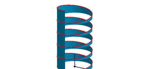
This example demonstrates the construction of a helix. It involves key mathematical concepts such as 3D vectors and parametric equations. Using GeoGebra commands like CurveCartesian, Surface, Segment, Midpoint, Translate, and Sequence, a helix can be constructed. Suitable for high school mathematics education and learning 3D geometry.
GeoGebra Commands & Parameters
CurveCartesian((-If[k ≤ 0.5, (((k * 2) * π) * r), (π * r)]) + If[t ≤ ((k * 2) * π), (t * r), (((k * 2) * π) * r) + (r * sin(t - ((k * 2) * π)))], (-r) + If[t ≤ ((k * 2) * π), 0, r - (r * cos(t - ((k * 2) * π)))], t, 0, (2 * π)) → aCurveCartesian((-If[k ≤ 0.5, (((k * 2) * π) * r), (π * r)]) + If[t ≤ ((k * 2) * π), (t * r), (((k * 2) * π) * r) + (r * sin(t - ((k * 2) * π)))], (-r) + If[t ≤ ((k * 2) * π), 0, r - (r * cos(t - ((k * 2) * π)))], h, t, 0, (2 * π)) → cCurveCartesian((-If[k ≤ 0.5, (((k * 2) * π) * r), (π * r)]) + If[t ≤ ((k * 2) * π), (t * r), (((k * 2) * π) * r) + (r * sin(t - ((k * 2) * π)))], (-r) + If[t ≤ ((k * 2) * π), 0, r - (r * cos(t - ((k * 2) * π)))], (h * t / 2 / π), t, 0, (2 * π)) → dSurface((-If[k ≤ 0.5, (((k * 2) * π) * r), (π * r)]) + If[t ≤ ((k * 2) * π), (t * r), (((k * 2) * π) * r) + (r * sin(t - ((k * 2) * π)))], (-r) + If[t ≤ ((k * 2) * π), 0, r - (r * cos(t - ((k * 2) * π)))], s, t, 0, (2 * π), s, 0, h) → bSegment(((-If[k ≤ 0.5, (((k * 2) * π) * r), (π * r)]), (-r) + 0, 0), ((-If[k ≤ 0.5, (((k * 2) * π) * r), (π * r)]), (-r) + 0, h)) → fSegment(((-If[k ≤ 0.5, (((k * 2) * π) * r), (π * r)]) + (((k * 2) * π) * r) + (r * sin((2 * π) - ((k * 2) * π))), (-r) + r - (r * cos((2 * π) - ((k * 2) * π))), 0), ((-If[k ≤ 0.5, (((k * 2) * π) * r), (π * r)]) + (((k * 2) * π) * r) + (r * sin((2 * π) - ((k * 2) * π))), (-r) + r - (r * cos((2 * π) - ((k * 2) * π))), h)) → gSegment((0, (-r), 0), (0, (-r), h)) → iSurface((v * c(u)) + ((1 - v) * d(u)), u, 0, (2 * π), v, 0, 1) → lSurface((v * a(u)) + ((1 - v) * d(u)), u, 0, (2 * π), v, 0, 1) → mMidpoint(f) → AMidpoint(g) → BMidpoint(A, B) → CTranslate(l, Vector[(Expand * Vector[C, C + (0, 0, Expand)])]) → l'Translate(d, Vector[(Expand * Vector[C, C + (0, 0, Expand)])]) → d'Translate(d, Vector[((2 * Expand) * Vector[C, C + (0, 0, Expand)])]) → d'_1Translate(m, Vector[((2 * Expand) * Vector[C, C + (0, 0, Expand)])]) → l'_1Sequence(Translate[d, Vector[((i * Expand) * Vector[C, C + (0, 0, Expand)])]], i, 0, n) → l1Sequence(Translate[m, Vector[((i * Expand) * Vector[C, C + (0, 0, Expand)])]], i, 0, n) → l2Segment((0, 0), (0, 0) + (r, 0, 0)) → jSegment(O, O + (0, 0, h)) → p
AI Drawing Prompt Reference
Draw a helix with radius r and height h, using the parametric equation x = r * t, y = r * (1 - cos(t)), z = r * (t - sin(t)) for t from 0 to 2π. Construct a helical surface with the parametric equation x = r * t * cos(u), y = r * t * sin(u), z = r * (t - sin(u)) for t from 0 to 2π and u from 0 to h. Draw two vertical line segments from the start and end points of the helix. Find the midpoint C of the helix, then translate the helical surface and helix along C by a distance of Expand. Finally, draw n equally spaced translated copies of the helix.
The prompt above was compiled from the original drawing commands and is for reference only.