Geostationary Satellites (Clarke Belt) 3D Orbit Demonstration

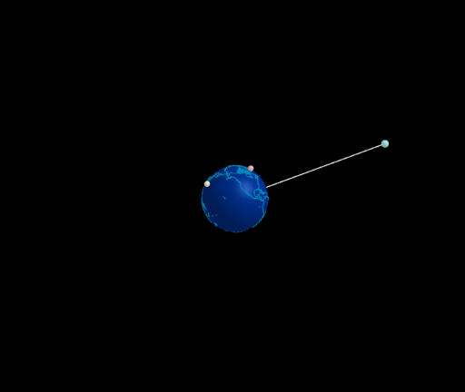
This GeoGebra example demonstrates the orbital configuration of geostationary satellites, known as the Clarke Belt, in a 3D space. It visualizes how satellites remain fixed relative to a point on Earth's equator by matching their orbital angular velocity with Earth's rotation. Core mathematical concepts include 3D vectors, circular motion, angular velocity, orbital radius, and the relationship between orbital period and geostationary altitude. The construction uses GeoGebra commands such as Sphere (to model Earth), Line and Circle (to draw orbital paths and reference axes), and Segment (to connect satellites to Earth's center). Sliders (ω, ω1, ω2, ω3) control angular speeds, while parameters like t, dt, tt drive animation. Multiple satellite objects (M1, M2, M3) with distinct orbital radii (a1, a2, a3) and distances (d1, d2, d3) are included, along with text labels for data display. This is suitable for high school physics or introductory astronomy/space engineering courses, helping students grasp synchronous orbits, the Clarke Belt concept, and 3D geometric modeling.