
Parametric Simulation of Uniform Circular Motion
Loading the math board and drawing, please wait…
In collections
The Domain of the Time (intuitive kinematics)
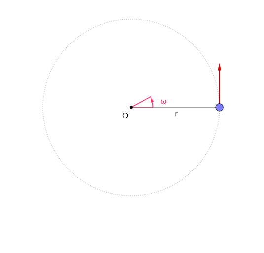
This GeoGebra applet demonstrates uniform circular motion dynamically. Core mathematical concepts include: parametric equations for circular motion, relationship between angular velocity and period, vector composition and decomposition (velocity direction always tangent to the circle). Construction: Circle command for the base circle, Segment for radius and trajectory, Angle for measuring rotation angle, If and mean for conditional statistics and mean calculations, Slider animation to show point P moving on the circle as parameter t (time) varies, displaying real-time physical quantities like linear velocity v, angular velocity ω, and period T. Suitable for high school physics lessons on uniform circular motion and mathematics teaching of parametric equations, helping students understand the directional relationship between velocity and acceleration in circular motion.
GeoGebra Commands & Parameters
Circle((0, 0), r) → cSegment(O, M) → sIf(Length[reg] ≟ 1, {reg(1)}, Sequence[reg(k) - reg(k + 1), k, 1, Length[reg] - 1]) → regDifmean(regDif) → TAngle((1, 0), O, Rotate[(1, 0), ω]) → αSegment(O, P) → f
AI Drawing Prompt Reference
Draw a circle with radius r centered at the origin. Draw a radius OM from the center. Use a slider to represent time t, and animate point P moving on the circle to show linear velocity v, angular velocity ω, and period T. Draw a vector from the center to P to represent the direction of velocity, which is always tangent to the circle. Calculate the rotation angle α using angular velocity ω and draw a vector from the center to P to represent the velocity direction.
The prompt above was compiled from the original drawing commands and is for reference only.