
Histogram Construction Tool: Frequency Counting and Distribution Parameters
Loading the math board and drawing, please wait…
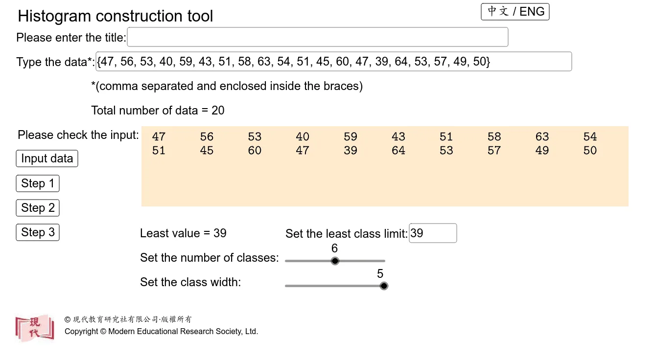
This example demonstrates how to automatically build a histogram in GeoGebra and visualize how the distribution shape emerges from frequency counts over integer values. Key concepts include histogram binning, frequency/statistical counting, and a discrete probability model (notably the binomial distribution) with parameters such as p and q, along with integer sample ranges. Construction-wise, the workflow determines the value bounds with Length, Min, and Max, then uses If together with CountIf to select and count data falling into each bin. Sequence is used to generate the required indices/integer values for binning, and Frequency aggregates the resulting counts. For presentation, Textfield and TableText manage labels and tabular outputs, while Append assembles the display elements. Finally, Segment and VerticalText are used to draw the vertical bars of the histogram and annotate them. Suitable for upper-secondary through early university probability & statistics, classroom demonstrations, and interactive exploration of how parameter changes affect empirical frequency patterns.
GeoGebra Commands & Parameters
Length(Data) → nMin(Data) → pMax(Data) → qIf(d > 1, 1, If[d > 0.1, 0.1, 0.01]) → tCountIf(A2 ≤ x ≤ C2, Data) → H2CountIf(A3 ≤ x ≤ C3, Data) → H3CountIf(A4 ≤ x ≤ C4, Data) → H4CountIf(A5 ≤ x ≤ C5, Data) → H5CountIf(A6 ≤ x ≤ C6, Data) → H6CountIf(A7 ≤ x ≤ C7, Data) → H7CountIf(A8 ≤ x ≤ C8, Data) → H8CountIf(A9 ≤ x ≤ C9, Data) → H9Sequence(a - t / 2 + ((i - 1) * d), i, 1, k + 1, 1) → BoundariesFrequency(Boundaries, Data) → FreqMax(ceil(Max[Freq] / b), 2) → uSequence(a - t / 2 + (((2 * i) - 1) * d / 2), i, 1, k, 1) → ClassMarkSequence((i * b), i, 2, u + 1, 2) → FreqMarkSequence((-8.5 - (0.25 * (ceil(lg(Element[FreqMark, i / 2] + 1)) - 1)), i - 4.15), i, 2, u + 1, 2) → YpointSequence((i - 8.15 - (0.15 * ceil(lg(Element[ClassMark, (i - 1) / 2] + 1) - 1)), -4.6), i, 3, 2 + (2 * k) - 1, 2) → XpointTextfield(Title) → InputBoxTitleTextfield(Data) → InputBoxDataTextfield(a) → InputBox3Sequence(If[n ≥ i, Element[Data, i], x], i, 1, If[n ≥ 10, 10, n], 1) → list1Sequence(If[n ≥ i, Element[Data, i], x], i, 11, If[n ≥ 20, 20, n], 1) → list2Sequence(If[n ≥ i, Element[Data, i], 32], i, 21, If[n ≥ 30, 30, n], 1) → list3Sequence(If[n ≥ i, Element[Data, i], x], i, 31, If[n ≥ 40, 40, n], 1) → list4Sequence(If[n ≥ i, Element[Data, i], x], i, 51, If[n ≥ 60, 60, n], 1) → list6Sequence(If[n ≥ i, Element[Data, i], x], i, 61, If[n ≥ 70, 70, n], 1) → list7Sequence(If[n ≥ i, Element[Data, i], x], i, 71, If[n ≥ 80, 80, n], 1) → list8Sequence(If[n ≥ i, Element[Data, i], x], i, 81, If[n ≥ 90, 90, n], 1) → list9Sequence(If[n ≥ i, Element[Data, i], x], i, 41, If[n ≥ 50, 50, n], 1) → list5Sequence(If[n ≥ i, Element[Data, i], x], i, 91, If[n ≥ 100, 100, n], 1) → list10TableText({list1, list2, list3, list4, list5, list6, list7, list8, list9, list10, "."}) → text21Append(Element[list11, 1], Sequence[Element[list21, i], i, 1, k, 1]) → list25Append(Element[list11, 2], Sequence[Element[list22, i], i, 1, k, 1]) → list26Append(Element[list11, 3], Sequence[Element[list23, i], i, 1, k, 1]) → list27Append(Element[list11, 4], Sequence[Element[list24, i], i, 1, k, 1]) → list28TableText({list25, list26, list27, list28}, "vc|_") → text22Sequence(Segment[(-8, (0.2 * i) - 4), (-5 + (2 * k), (0.2 * i) - 4)], i, 1, ((u + 1) * 5), 1) → Hori1Sequence(Segment[(-8, i - 4), (-5 + (2 * k), i - 4)], i, 0, u + 1, 1) → Hori2Segment((-7.2, -3.6), (-7, -4.4)) → hSegment((-7.4, -4), (-7.2, -3.6)) → gSegment((-8.2, -4), (-7.4, -4)) → fSegment((-8, -4), (-8, u - 3)) → YaxisSegment((-6.8, -4), (-5 + (2 * k), -4)) → XaxisSegment((-7, -4.4), (-6.8, -4)) → iSequence(Segment[(-8, i - 4), (-8.2, i - 4)], i, 2, u + 1, 2) → Hori3Sequence(Segment[(i - 8, -4), (i - 8, u - 3)], i, 1, 2 + (2 * k) + 1, 1) → Vert2Sequence(Segment[(i - 8, -4), (i - 8, -4.2)], i, 3, 2 + (2 * k) - 1, 2) → Vert3Sequence(Polygon[(-6 + (2 * (i - 1)), -4), (-6 + (2 * (i - 1)), -4 + Element[Freq, i] / b), (-6 + (2 * i), -4 + Element[Freq, i] / b), (-6 + (2 * i), -4)], i, 1, k, 1) → BlockSequence(Segment[((0.2 * i) - 8, -4), ((0.2 * i) - 8, u - 3)], i, 1, ((2 + (2 * k) + 1) * 5), 1) → Vert1VerticalText(If[chi ≟ true, "頻 數", "Frequency"]) → text17
AI Drawing Prompt Reference
Draw a histogram showing frequency distribution of data. Determine data range from min and max, generate intervals via sequence, count frequencies per bin, then draw vertical bars with heights equal to frequencies. Label intervals and frequencies on the left, and annotate the right. Construction order: set range and bin width, count frequencies, then draw bars and labels.
The prompt above was compiled from the original drawing commands and is for reference only.