
High School Frog Population Tracking GeoGebra Example
Loading the math board and drawing, please wait…
In collections
CCGPS AA Unit 6 Lesson 5
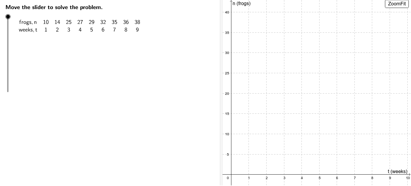
This example demonstrates how to use GeoGebra to track and visualize the population changes of tree frogs in a cypress tree over 9 weeks by a high school nature club. It involves core math concepts like sequences, linear equations, data fitting, and statistical analysis. Constructed using commands like Length, LaTeX, Corner, TableText, Sequence, Fit, Sum, If, and objects such as frogs, numpts, stepMax, etc., it visualizes dynamic data input, processing, and representation. Suitable for high school mathematics education, showcasing the application of data modeling and function fitting.
GeoGebra Commands & Parameters
Length(frogs) → numptsLaTeX(steps) → counterLaTeX("\text{Move the slider to solve the problem.}") → text0Corner(1) → ACorner(3) → BTableText({{"frogs,n", Element[frogs, 1], Element[frogs, 2], Element[frogs, 3], Element[frogs, 4], Element[frogs, 5], Element[frogs, 6], Element[frogs, 7], Element[frogs, 8], Element[frogs, 9]}, {"weeks,t", 1, 2, 3, 4, 5, 6, 7, 8, 9}}, "c") → tableLaTeX(table) → ProblemLaTeX("\text{Create a scatter plot of the table values.}") → text1Sequence((i, Element[frogs, i]), i, 1, numpts) → plotFit(plot, (a * b^(x))) → fFit(plot, (c * x^(d))) → gLaTeX(g, true, true) → text6LaTeX("\text{Which function fits the data best?}") → text7Sequence((Element[frogs, i] - f(i))^(2), i, 1, numpts) → fdiffsSequence((Element[frogs, i] - g(i))^(2), i, 1, Length[frogs]) → gdiffsSum(fdiffs) → fmsSum(gdiffs) → gmsLaTeX("\text{Fit an exponential function of the form }\textcolor{#006633}{f(x) = a b^x}\text{ to the data.}") → text3LaTeX("\text{Fit a power function of the form }\textcolor{#CC0000}{g(x) = c x^d}\text{ to the data.}") → text5LaTeX("\text{Does the shape of the function look similar to the shape of the data}\cr\text{or does the function appear to be headed off in a different direction}\cr\text{from the data?}") → text8LaTeX("\text{Is one function consistently closer to the individual data points than the other?}") → text10LaTeX("\text{Do the functions do anything obviously unreasonable if they are used }\cr\text{to predict values {outside the range of collected data?}") → text12LaTeX("\text{Neither function does this. We know in general that exponential }\cr\text{growth cannot occur indefinitely, but that it does occur temporarily.}") → text13LaTeX("\text{Use the buttons below to return to the original problem or}\cr\text{randomly generate a similar practice problem.}") → RandomizationTextIf(angleMargin < (-0.2), LaTeX["\text{The }\textcolor{#006633}{exponential} \text{ function does better with this.}"], If[angleMargin > 0.2, LaTeX["\text{The }\textcolor{#CC0000}{power}\text{ function does better with this.}"], LaTeX["\text{The functions are similar in this respect.}"]]) → text9If(margin < (-0.2), LaTeX["\text{The }\textcolor{#006633}{exponential}\text{ function does better with this.}"], If[margin > 0.2, LaTeX["\text{The }\textcolor{#CC0000}{power}\text{ function does better with this.}"], LaTeX["\text{The functions are similar in this respect.}"]]) → text11LaTeX("\text{Data points should not be connected by any lines.}") → text2LaTeX((("\textcolor{#006633}{f(x)=" * f) * "} \text{ Note: functions may vary.}")) → text4Length(frogs_1) → numpts_1Sequence((i, Element[frogs_1, i]), i, 1, numpts_1) → plot_1Fit(plot_1, (a * b^(x))) → f_1LaTeX("\text{ Note: functions may vary.}") → text4_1
AI Drawing Prompt Reference
Create a high school frog population tracking visualization showing the number of tree frogs over 9 weeks. Include a scatter plot for actual data points, and two fitted curves (exponential and power functions) to compare their fit. The chart should feature a data table, explanatory text, and function expressions to analyze which model better represents the population growth trend.
The prompt above was compiled from the original drawing commands and is for reference only.