
Heaviside & Dirac Delta Functions
Loading the math board and drawing, please wait…
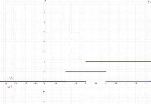
This example demonstrates the graphs and properties of the Heaviside and Dirac delta functions, which are important in signal processing and physics. By adjusting parameters, you can observe the changes in the functions. This example uses GeoGebra commands such as Textfield, InputBox, showheavy, and showdirac, suitable for students in university mathematics and engineering.
GeoGebra Commands & Parameters
Textfield(a) → InputBox1Textfield(deltatmin) → InputBox2Textfield(deltatmax) → InputBox3
AI Drawing Prompt Reference
Create a coordinate plot illustrating the Heaviside step function and the Dirac delta function. The horizontal axis represents time, and the vertical axis shows function values. Include two adjustable input boxes for setting the minimum and maximum time range of the delta function. The step function jumps from 0 to 1 at the origin, while the delta function appears as a sharp spike at the origin, with its height and width varying with the parameters. Clearly label both curves and show how they change with different parameter values, highlighting their key properties in signal processing.
The prompt above was compiled from the original drawing commands and is for reference only.