
Geogebra Calculus & Optimization Demo
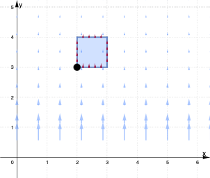
Loading the math board and drawing, please wait…
This example dynamically demonstrates calculus optimization problems using GeoGebra, integrating function graphs, derivatives, and polygon constructions. Core concepts include derivatives, optimization, polygon construction, and function graphing. It utilizes commands like Polygon, CurveCartesian, Textfield, Sequence, Derivative, Sum, Centroid, and LaTeX. Suitable for high school and above students studying calculus, coordinate geometry, and optimization.
GeoGebra Commands & Parameters
Polygon(A1, A2, A3, A4) → P1, a1, a2, a3, a4CurveCartesian((t * x(A2)) + ((1 - t) * x(A1)), (t * y(A2)) + ((1 - t) * y(A1)), t, 0, 1) → c1CurveCartesian((t * x(A3)) + ((1 - t) * x(A2)), (t * y(A3)) + ((1 - t) * y(A2)), t, 0, 1) → c2CurveCartesian((t * x(A4)) + ((1 - t) * x(A3)), (t * y(A4)) + ((1 - t) * y(A3)), t, 0, 1) → c3CurveCartesian((t * x(A1)) + ((1 - t) * x(A4)), (t * y(A1)) + ((1 - t) * y(A4)), t, 0, 1) → c4Textfield(F_1) → FxTextfield(F_2) → FySequence(Sequence[Vector[(j, k), (j + (scale * F_1(j, k)), k + (scale * F_2(j, k)))], j, xmin, xmax, xstep], k, ymin, ymax, ystep) → field, {{(NaN, NaN), (NaN, NaN), (NaN, NaN), (NaN, NaN), (NaN, NaN), (NaN, NaN), (NaN, NaN), (NaN, NaN), (NaN, NaN), (NaN, NaN)}, {(0, 0.5999692364897973), (0, 0.5999692364897973), (0, 0.5999692364897973), (0, 0.5999692364897973), (0, 0.5999692364897973), (0, 0.5999692364897973), (0, 0.5999692364897973), (0, 0.5999692364897973), (0, 0.5999692364897973), (0, 0.5999692364897973)}, {(0, 0.29998461824489864), (0, 0.29998461824489864), (0, 0.29998461824489864), (0, 0.29998461824489864), (0, 0.29998461824489864), (0, 0.29998461824489864), (0, 0.29998461824489864), (0, 0.29998461824489864), (0, 0.29998461824489864), (0, 0.29998461824489864)}, {(0, 0.1999897454965991), (0, 0.1999897454965991), (0, 0.1999897454965991), (0, 0.1999897454965991), (0, 0.1999897454965991), (0, 0.1999897454965991), (0, 0.1999897454965991), (0, 0.1999897454965991), (0, 0.1999897454965991), (0, 0.1999897454965991)}, {(0, 0.1499923091224491), (0, 0.1499923091224491), (0, 0.1499923091224491), (0, 0.1499923091224491), (0, 0.1499923091224491), (0, 0.1499923091224491), (0, 0.1499923091224491), (0, 0.1499923091224491), (0, 0.1499923091224491), (0, 0.1499923091224491)}, {(0, 0.11999384729795937), (0, 0.11999384729795937), (0, 0.11999384729795937), (0, 0.11999384729795937), (0, 0.11999384729795937), (0, 0.11999384729795937), (0, 0.11999384729795937), (0, 0.11999384729795937), (0, 0.11999384729795937), (0, 0.11999384729795937)}, {(0, 0.09999487274829955), (0, 0.09999487274829955), (0, 0.09999487274829955), (0, 0.09999487274829955), (0, 0.09999487274829955), (0, 0.09999487274829955), (0, 0.09999487274829955), (0, 0.09999487274829955), (0, 0.09999487274829955), (0, 0.09999487274829955)}, {(0, 0.0857098909271139), (0, 0.0857098909271139), (0, 0.0857098909271139), (0, 0.0857098909271139), (0, 0.0857098909271139), (0, 0.0857098909271139), (0, 0.0857098909271139), (0, 0.0857098909271139), (0, 0.0857098909271139), (0, 0.0857098909271139)}, {(0, 0.07499615456122477), (0, 0.07499615456122477), (0, 0.07499615456122477), (0, 0.07499615456122477), (0, 0.07499615456122477), (0, 0.07499615456122477), (0, 0.07499615456122477), (0, 0.07499615456122477), (0, 0.07499615456122477), (0, 0.07499615456122477)}, {(0, 0.06666324849886607), (0, 0.06666324849886607), (0, 0.06666324849886607), (0, 0.06666324849886607), (0, 0.06666324849886607), (0, 0.06666324849886607), (0, 0.06666324849886607), (0, 0.06666324849886607), (0, 0.06666324849886607), (0, 0.06666324849886607)}}Derivative(c1) → dc1Derivative(c2) → dc2Derivative(c3) → dc3Derivative(c4) → dc4Sum(Sequence[(((F_1(x(c1(i + dS / 2)), y(c1(i + dS / 2))), F_2(x(c1(i + dS / 2)), y(c1(i + dS / 2)))) * (y(dc1(i + dS / 2)), (-x(dc1(i + dS / 2))))) * dS), i, 0, s - dS, dS]) → Flux1Sum(Sequence[(((F_1(x(c2(i + dS / 2)), y(c2(i + dS / 2))), F_2(x(c2(i + dS / 2)), y(c2(i + dS / 2)))) * (y(dc2(i + dS / 2)), (-x(dc2(i + dS / 2))))) * dS), i, 0, s - dS, dS]) → Flux2Sum(Sequence[(((F_1(x(c3(i + dS / 2)), y(c3(i + dS / 2))), F_2(x(c3(i + dS / 2)), y(c3(i + dS / 2)))) * (y(dc3(i + dS / 2)), (-x(dc3(i + dS / 2))))) * dS), i, 0, s - dS, dS]) → Flux3Sum(Sequence[(((F_1(x(c4(i + dS / 2)), y(c4(i + dS / 2))), F_2(x(c4(i + dS / 2)), y(c4(i + dS / 2)))) * (y(dc4(i + dS / 2)), (-x(dc4(i + dS / 2))))) * dS), i, 0, s - dS, dS]) → Flux4Centroid(P1) → C1Derivative(F_1, x) → dxF_1Derivative(F_2, y) → dyF_2LaTeX(divVal, true, true) → text1Sequence(Vector[c1(s), c1(s) + ((scale * F_1(x(c1(s)), y(c1(s)))), (scale * F_2(x(c1(s)), y(c1(s)))))], s, 0.2, 0.8, 0.2) → vect1Sequence(Vector[c3(s), c3(s) + ((scale * F_1(x(c3(s)), y(c3(s)))), (scale * F_2(x(c3(s)), y(c3(s)))))], s, 0.2, 0.8, 0.2) → vect3Sequence(Vector[c4(s), c4(s) + ((scale * F_1(x(c4(s)), y(c4(s)))), (scale * F_2(x(c4(s)), y(c4(s)))))], s, 0.2, 0.8, 0.2) → vect4Sequence(Vector[c2(s), c2(s) + ((scale * F_1(x(c2(s)), y(c2(s)))), (scale * F_2(x(c2(s)), y(c2(s)))))], s, 0.2, 0.8, 0.2) → vect2
AI Drawing Prompt Reference
Draw a quadrilateral ABCD, connect its diagonals AC and BD. Take points E, F, G, H on AB, BC, CD, DA respectively, such that AE=EB, BF=FC, CG=GD, DH=HA. Draw the perpendicular bisectors of AB, BC, CD, DA, and mark the centroid of the quadrilateral. Calculate and display the area of the quadrilateral. Draw the gradient field of the quadrilateral.
The prompt above was compiled from the original drawing commands and is for reference only.