
Heat Equation Demonstration
Loading the math board and drawing, please wait…
In collections
UQ-Applied Mathematical Analysis
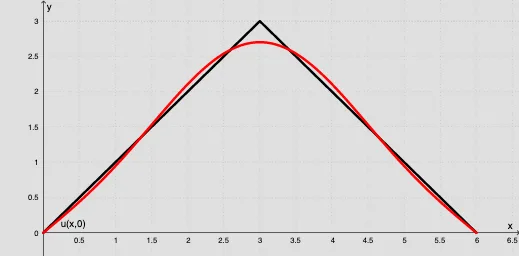
This example dynamically visualizes the solution and evolution of the heat equation using geometric constructions. Key math concepts include partial differential equations, numerical methods, vector fields, and function graphing. The construction summary employs commands like Sequence, Max/Min, Textfield, Vector, OrthogonalLine, If, Polygon, Sum, LaTeX, and CurveCartesian. Ideal for high school students and math enthusiasts studying PDEs and numerical simulations.
GeoGebra Commands & Parameters
Sequence(g(i), i, 0, L, 0.1) → list1Max(list1) → maxlist1Min(list1) → minlist1Textfield(f) → InputBox1Vector(A, B) → uVector(A, C) → vOrthogonalLine(C, yAxis) → hOrthogonalLine(B, yAxis) → iIf(y(v) > 0, 0, 1) → condyIf(y(u) < 0, 0, 1) → condxIf(ymin ≟ 0, (ymax * (-0.1)), ymin) → condy2If(ymax ≟ 0, (ymin * (-0.1)), ymax) → condx2Textfield(L) → InputBox2Polygon((xmin1, ymin1), ((-0.1 * L), ymin1), ((-0.1 * L), ymax1), (xmax1, ymax1)) → Range1, j, k, l, mPolygon((xmin2, ymin2), (L, ymin2), (L, ymax2), (xmax2, ymax2)) → Range2, p, q, r, sSequence((2 / L * Integral[(f(x) * sin((((π * x) * i)) / L)), 0, L]), i, 1, n) → AnSequence(((Element[An, i] * exp(((((-a) * i^(2)) * π^(2)) * y / L^(2)))) * sin(((i * π) * x / L))), i, 1, n) → AnexpsinSum(Anexpsin, n) → vvTextfield(a) → InputBox3Textfield(n) → InputBox4If(t < 30, t, 30) → hueLaTeX(hue, true, true) → text1CurveCartesian(o, heat(o), o, 0, L) → c
AI Drawing Prompt Reference
Create a dynamic visualization of the heat equation solution. On a coordinate plane, draw a curve representing temperature distribution that evolves with a parameter. Include several input boxes for adjusting the initial function, domain length, thermal diffusivity, and number of series terms. Mark the solution domain with two rectangular regions. Add two vectors indicating directions and a vertical auxiliary line. The curve is formed by summing sinusoidal terms with coefficients from integrals, each decaying exponentially with time. Use color mapping to indicate time progression and display the current time value. The layout should be clear for educational demonstration.
The prompt above was compiled from the original drawing commands and is for reference only.