Graphs of Exponential Function y = k a^x: Parameter Exploration

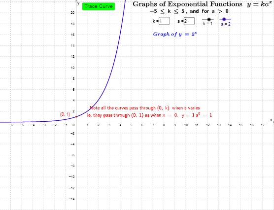
This GeoGebra example demonstrates the graphs of the exponential function y = k a^x and how the coefficient k and base a influence the curve’s shape, position, growth, and decay. It is designed for self-learning and classroom demonstration of exponential functions. Key mathematical concepts include exponential functions, function transformations, vertical stretching and compressing, horizontal scaling, asymptotic behavior, and the distinction between exponential growth (a > 1) and exponential decay (0 < a < 1). The construction relies on GeoGebra commands and objects such as Point, Textfield, inputBox, button, and text objects text1, text3, text4, text5, text6, text7, text8 for dynamic parameter display, together with f and f_{trace} for plotting the function graph and its trace, and variables a, k, b, c, q1, q2, C linked to interactive controls. Suitable for high school mathematics, teachers, and students exploring function graphs and parameter effects.