
Graphing Exponential Functions y = k a^x
Loading the math board and drawing, please wait…
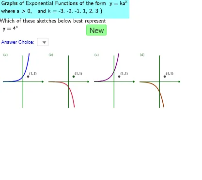
This example demonstrates how to graph exponential functions y = k a^x. Key mathematical concepts include the properties and graph characteristics of exponential functions. Using GeoGebra commands such as Simplify and Shuffle, you can dynamically adjust parameters k and a to observe changes in the graph. Suitable for high school math education and learning.
GeoGebra Commands & Parameters
Simplify((RandomElement[liste_a]^(x) * Element[liste_k, 1])) → F12Simplify((RandomElement[liste_a]^(x) * Element[liste_k, 3])) → F11Simplify((RandomElement[liste_a]^(x) * Element[liste_k, 2])) → F10Simplify((RandomElement[liste_a]^(x) * Element[liste_k, 1])) → F9Shuffle({9, 11, 13, 15}) → listshowGf1, {13, 11, 15, 9}Shuffle({10, 12, 14, 16}) → listshowGf2, {16, 14, 12, 10}Shuffle({9, 10, 13, 14}) → listshowGf3, {9, 14, 13, 10}Shuffle({11, 12, 15, 16}) → listshowGf4, {16, 15, 11, 12}Shuffle({9, 12, 13, 16}) → listshowGf5, {13, 9, 12, 16}Shuffle({10, 11, 14, 15}) → listshowGf6, {14, 11, 10, 15}Sequence(If[count < 3, Element[listshowGf0, i], If[count < 5, Element[listshowGf1, i], If[count < 7, Element[listshowGf2, i], If[count < 9, Element[listshowGf3, i], If[count < 11, Element[listshowGf4, i], If[count < 11, Element[listshowGf5, i], Element[listshowGf6, i]]]]]]], i, 1, 4) → listnsGIf(useG, If[count > 2, Random[0, 7], 3], Random[0, 7]) → e'Random(1, 4) → dIf(count > 2, Random[1, 4], If[count > 1, 3, 1]) → n_gIf(d ≟ e' ∧ (count > 8 ∨ count < 5), 1, e') → eRandom(1, 4) → n_fShuffle({1, 2, 3, 4}) → listshowFf1, {4, 1, 3, 2}Shuffle({1, 4, 5, 8}) → listshowFf2a, {1, 8, 4, 5}Shuffle({2, 3, 6, 7}) → listshowFf2b, {6, 2, 3, 7}If(count < 5, Element[listFf, Element[listshowFf1, 3]], If[count < 9, Element[listFf, Element[listshowFf2a, 3]], Element[listFf, Element[listshowFf2b, 3]]]) → f_{3s}Coefficients(f_{3s}) → listf_{3s}If(count < 5, Element[listFf, Element[listshowFf1, 4]], If[count < 9, Element[listFf, Element[listshowFf2a, 4]], Element[listFf, Element[listshowFf2b, 4]]]) → f_{4s}Coefficients(f_{4s}) → listf_{4s}If(count < 5, Element[listFf, Element[listshowFf1, 1]], If[count < 9, Element[listFf, Element[listshowFf2a, 1]], Element[listFf, Element[listshowFf2b, 1]]]) → f_{1s}Coefficients(f_{1s}) → listf_{1s}If(count < 5, Element[listFf, Element[listshowFf1, 2]], If[count < 9, Element[listFf, Element[listshowFf2a, 2]], Element[listFf, Element[listshowFf2b, 2]]]) → f_{2s}Coefficients(f_{2s}) → listf_{2s}Element(listCoeffs, n_f, 1) → a_fElement(listCoeffs, n_f, 2) → b_fSimplify((-F9(x))) → F13Simplify((-F10(x))) → F14Simplify((-F11(x))) → F15Simplify((-F12(x))) → F16Sequence(Sequence[(x(A) + (s_p * i), y(A) + (s_p * j)), i, 0, 3], j, 0, 0) → list3CtrofGraphs, {{(5, 0), (13.8, 0), (22.6, 0), (31.400000000000002, 0)}}Polygon(E, D, F, G) → poly2, e_1, d_1, f_5, gPolygon(J, K, L, M) → poly4, j, k, l, mPolygon(J, K, C, B) → poly5, j_1, k_1, c, b_1Sequence(Sequence[Segment[(x(A) + (s_p * i) - l_x / 2, y(A) + (s_p * j)), (x(A) + (s_p * i) + l_x / 2, y(A) + (s_p * j))], i, 0, 3], j, 0, 0) → list1Xaxes, {{7.6000000000000005, 7.600000000000001, 7.600000000000001, 7.600000000000001}}Sequence(Sequence[Segment[(x(A) + (s_p * i), y(A) + (s_p * j) - l_y / 2), (x(A) + (s_p * i), y(A) + (s_p * j) + l_y / 2)], i, 0, 3], j, 0, 0) → list2Yaxes, {{10, 10, 10, 10}}Sequence(Sequence[(x(A) + l_x / 2 + (s_p * i), y(A) + (s_p * j)), i, 0, 3], j, 0, 0) → listXarrow, {{(8.8, 0), (17.6, 0), (26.400000000000002, 0), (35.2, 0)}}Sequence(Sequence[Text[Element[listChoicestext, i + 1], (x(A) - l_x / 2 + (s_p * (i - 1)), y(A) + l_y / 2)], i, 1, 4], j, 0, 0) → listChoicestextDisplay, {{"(a)", "(b)", "(c)", "(d)"}}Element(listCoeffs, n_f, 3) → c_fIf(useG, x(Element[listTurningPointsG, Element[listnsG, n_g] - 8]), ((-b_f)) / ((2 * a_f))) → symx2Defined(root1) → realrootsIf(count < 5, Element[listFf, Element[listshowFf1, 4]], If[count < 9, Element[listFf, Element[listshowFf2a, 4]], Element[listFf, Element[listshowFf2b, 4]]]) → f_{tests}Polygon(B, C, D, E) → poly1, b, c_1, d_2, e_2If(count < 5, Element[listshowFf1, n_f], If[count < 9, Element[listshowFf2a, n_f], Element[listshowFf2b, n_f]]) → n_sSequence(If[count < 5, Element[listshowFf1, i], If[count < 9, Element[listshowFf2a, i], Element[listshowFf2b, i]]], i, 1, 4) → listnsFMin(d, e) → I1Min((-d), e) → I2Min(d, (-e)) → I3Min((-d), (-e)) → I4Min(d, e) → I5Min((-d), e) → I6Min(d, (-e)) → I7Min((-d), (-e)) → I8Max(d, e) → J1Max((-d), e) → J2Max((-d), e) → J6Max(d, (-e)) → J7Max(d, (-e)) → J3Max((-d), (-e)) → J4Max(d, e) → J5Max((-d), (-e)) → J8Element(listGf, Element[listnsG, 1] - 8) → g_{1s}Element(listGf, Element[listnsG, 2] - 8) → g_{2s}Element(listGf, Element[listnsG, 4] - 8) → g_{4s}Element(listGf, Element[listnsG, 3] - 8) → g_{3s}Sequence((0, Cell[7, 8 + i]), i, 1, 8) → listyinterceptsElement(Coefficients[Simplify[Cell[6, Element[listnsG, n_g]]]], 2) → b_gElement(Coefficients[Simplify[Cell[6, Element[listnsG, n_g]]]], 3) → c_gElement(Coefficients[Simplify[Cell[6, Element[listnsG, n_g]]]], 1) → a_gIntersect(f_{1one}, f_{12minusx}) → N
AI Drawing Prompt Reference
Draw the graphs of exponential functions y = k a^x to show how changing parameters k and a affects the graphs. Start by plotting three different exponential function graphs, each with unique k and a values. Then add x and y axes to the coordinate system and label them (a), (b), (c), (d) on the x-axis. Finally, plot the axis of symmetry and vertex of the functions based on their coefficients, and label key points.
The prompt above was compiled from the original drawing commands and is for reference only.