
Graphing Absolute Value of a Linear Function with Random Practice
Loading the math board and drawing, please wait…
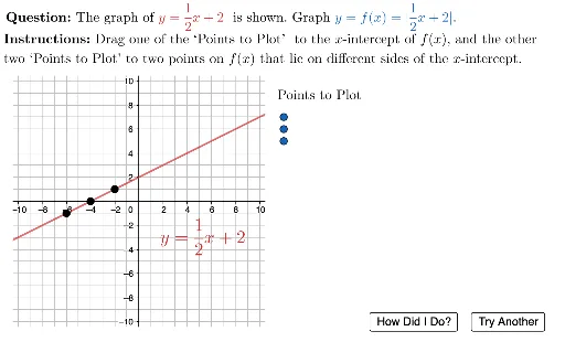
① This example demonstrates how to graph the absolute value of a linear function y = |mx + b|, with randomly generated parameters for interactive practice. ② Core math concepts include the V-shaped graph of absolute value functions, slope and intercept of linear functions, x-intercepts, and graphing using key points such as the vertex and intercepts. ③ Construction highlights: from the summary, it uses Random and Element to select random parameters, If and Intersect to compute intersections, Zip, Sort, Flatten to manage point lists, Point and Polygon to construct key points and shapes, LaTeX for formula display, Ray for drawing rays, and many interactive objects (buttons, feedback marks) for self-assessment. ④ Suitable for middle or high school algebra classes or self-study, helping students understand the graph of absolute value functions and practice sketching graphs from function expressions.
GeoGebra Commands & Parameters
Random(1, 10) → aIndxElement(aValLst, aIndx) → mValIf(abs(mVal) ≥ 1 / 2, Random[-4, 4], If[abs(mVal) ≤ 1 / 4, Random[-1, 1], Random[-2, 2]]) → bValIntersect(g, xAxis) → XinterceptPtZip((A, f(A)), A, keyPtxVals) → keyPointsGElement(keyPointsG, 2) → vertexPointSort(userPts) → userPtsSortedElement(userPtsSorted, 2) → UserPtMiddleZip((A, g(A)), A, keyPtxVals) → keyPointsFFlatten(Sequence[Sequence[(i, j), i, -10, 10], j, -10, 10]) → gridSpacePoint(Join[{gridSpace, keyPointsF, keyPointsG, {Element[homeBase, 2]}}]) → B3Point(Join[{gridSpace, keyPointsF, keyPointsG, {Element[homeBase, 1]}}]) → B2Point(Join[{gridSpace, keyPointsF, keyPointsG, {Element[homeBase, 3]}}]) → B4UnicodeToLetter(10007) → xmarkUnicodeToLetter(10003) → cmarkPolygon({bottomLeft, (x(bottomLeft), y(topRight)), topRight, (x(topRight), y(bottomLeft))}) → viewboxLaTeX(((("\vphantom{\dfrac{1}{1}}" * Element[aValFmt, aIndx]) * "x") * If[bVal ≟ 0, "", If[bVal < 0, ("" * bVal), ("+" * bVal)]])) → basicExprLaTeX((((("\text{\textbf{Question: }The graph of \textcolor{#d32f2f}{\(y=" * basicExpr) * "\) } is shown. Graph \textcolor{#1565c0}{\(y=f(x)=\vert") * basicExpr) * "\vert\)}. ")) → MainInstrucLaTeX((("f(x) = \mid" * basicExpr) * "\mid")) → lblAbsFuncLaTeX(("y=" * basicExpr)) → lblLinearFuncLaTeX((((((("\text{Any point on \(y=" * basicExpr) * "\) whose \(y\)-value \\is \(0\) or positive will also be on \\\(f(x)=\mid") * basicExpr) * "\mid\). \\Any point on \(y=") * basicExpr) * "\) whose \(y\)-value \\is negative will be reflected in the \(x\)-axis.}")) → fbExplanationElement(userPtsSorted, 1) → UserPtLeftElement(userPtsSorted, 3) → UserPtRightRay(UserPtMiddle, UserPtRight) → arm_1Ray(UserPtMiddle, UserPtLeft) → arm_2LaTeX("\text{\textbf{Instructions: }Drag one of the `Points to Plot' to the \(x\)-intercept of \(f(x)\), and the other \\two `Points to Plot' to two points on \(f(x)\) that lie on different sides of the \(x\)-intercept.}") → SpecInstruc
AI Drawing Prompt Reference
Draw the graph of an absolute value linear function y = |mx + b| with randomly generated m and b. Highlight the V-shaped graph, vertex, and x-intercepts. Use grid points and key points to plot the function, labeling the vertex and intercepts. Add interactive buttons allowing users to drag points to determine key points on the graph, with correct formulas and explanations displayed.
The prompt above was compiled from the original drawing commands and is for reference only.