
Gram-Schmidt Orthogonalization Process
Loading the math board and drawing, please wait…
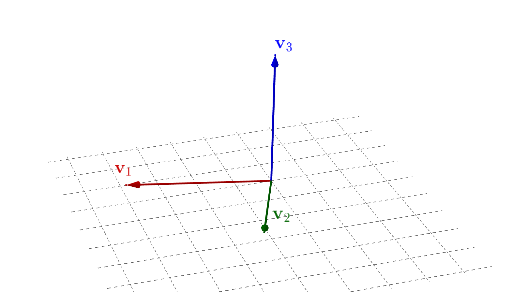
This example visualizes the Gram-Schmidt orthogonalization process, which transforms a set of vectors into a set of orthogonal vectors. Key mathematical concepts include vectors, orthogonality, and basis transformation. Using GeoGebra commands such as Vector, Sequence, Angle, etc., the orthogonalization process is demonstrated visually. Suitable for linear algebra courses at the university level.
GeoGebra Commands & Parameters
Vector(A) → e_1Vector(B) → e_2Vector(C) → e_3Sequence(Max[0, Min[1, k - s]], s, 0, top - 1) → slSequence(0 < sl(s) < 1, s, 1, top) → scSequence(0 < sl(s) ≤ 1, s, 1, top) → sc'MatrixRank(M) → condIf(0 ≤ k ≤ 1, (B * (1 - k)) + (P1 * k), P1) → T1If(1 ≤ k ≤ 2, (B * (1 - (k - 1))) + ((x(w2), y(w2), z(w2)) * (k - 1)), (x(w2), y(w2), z(w2))) → O1Vector(B, O1) → Vec2If(3 ≤ k ≤ 4, (C * (1 - (k - 3))) + (P2 * (k - 3)), P2) → T2Segment(T1, B) → S1Segment(T2, C) → S2If(4 ≤ k ≤ 5, (C * (1 - (k - 4))) + (Q2 * (k - 4)), Q2) → O2If(5 ≤ k ≤ 6, (Q2 * (1 - (k - 5))) + (P3 * (k - 5)), P3) → T3Segment(T3, Q2) → S3Vector((0, 0, 0), O2) → Vec3If(6 ≤ k ≤ 7, (Q2 * (1 - (k - 6))) + (Q3 * (k - 6)), Q3) → O3Vector((0, 0, 0), O3) → Vec4OrthogonalPlane((0, 0, 0), Vector[pv31 ⊗ pv32]) → planeAngle(w1, w2) → angle1Angle(w2, w3) → angle2Angle(w1, w3) → angle3If(7 ≤ k ≤ 8, Vector[(w1 * (1 - (k - 7))) + (Nw1 * (k - 7))], w1) → K1If(7 ≤ k ≤ 8, Vector[(w2 * (1 - (k - 7))) + (Nw2 * (k - 7))], w2) → K2If(7 ≤ k ≤ 8, Vector[(w3 * (1 - (k - 7))) + (Nw3 * (k - 7))], w2) → K3LaTeX(k, true, true) → text1LaTeX(vall, true, true) → text2Vector((0, 0, 0), O1) → w2'
AI Drawing Prompt Reference
This is a graphic showing the Gram-Schmidt orthogonalization process. It includes three initial vectors that are progressively orthogonalized. The process demonstrates how vectors are transformed into orthogonal vectors through a series of steps. The graphic also shows angle measurements and representations of orthogonal planes to help understand vector transformations. The construction order starts with the original vectors and proceeds with orthogonalization steps, ultimately yielding an orthogonal vector set.
The prompt above was compiled from the original drawing commands and is for reference only.