
Geometric Interpretation of Average vs. Instantaneous Rate of Change
Loading the math board and drawing, please wait…
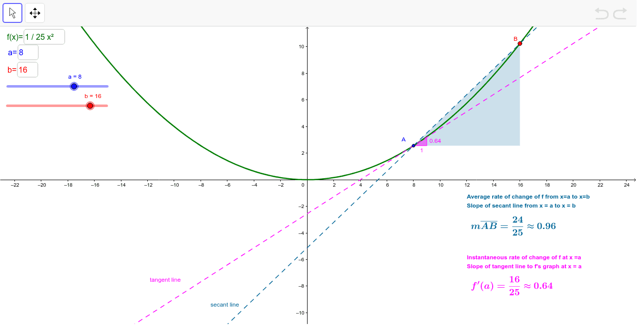
This example demonstrates the geometric interpretations of the average and instantaneous rates of change of a function f over an interval [a, b]. Key math concepts include average rate of change, instantaneous rate of change, slope, tangent, and function graphs. Constructed using GeoGebra commands like Textfield, Line, Intersect, Segment, Polygon, Slope, FractionText, Tangent. Suitable for high school and above students to understand fundamental calculus concepts and their geometric applications.
GeoGebra Commands & Parameters
Textfield(f) → InputBox1Textfield() → InputBox2Textfield(a) → InputBox3Line(A, B) → b_1Intersect(c, d) → CSegment(B, C) → eSegment(C, A) → gTextfield(b) → InputBox4Polygon(B, C, A) → poly1, a_1, b_2, c_1Slope(b_1) → iFractionText(i) → text1Tangent(A, f) → jSlope(j) → kFractionText(k) → text3
AI Drawing Prompt Reference
Draw the graph of function f over the interval [a, b] to illustrate average and instantaneous rates of change. Start by drawing the line segment between points a and b, then find the midpoint C and connect AC and BC to form a triangle. Next, draw the tangent line to f at point a and label its slope as the instantaneous rate of change.
The prompt above was compiled from the original drawing commands and is for reference only.