Geometric Construction for the Volume of a Sphere

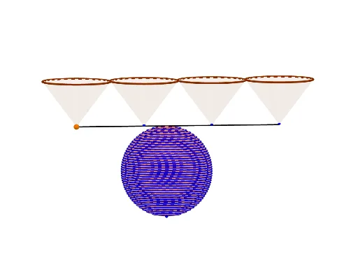
This example demonstrates how to compute and visualize the volume of a sphere by using a geometric construction based on parameterized slicing. It shows how the sphere’s volume can be interpreted as an accumulation of cross-sectional measures as the slicing parameter changes, connecting discrete approximations to an integral/limit viewpoint. The core math concepts include solid geometry (sphere volume), cross-section method, and numerical/sequence-based approximation of an integral via limiting behavior. Construction highlights: it uses GeoGebra commands Sphere and Cone to build the sphere and moving cone-like cross-sections, Sequence to generate parameter values t and the corresponding slice locations/sizes, and IntersectPath together with Segment to compute intersection points along a constructed path and to form the cross-sectional geometry used for volume accumulation. The example is suitable for high school to early university learners, especially for teaching and intuition-building around solid geometry and calculus ideas such as integral approximation and limits.