
Geometric Centers on a Sphere Induced by Moving Points in 3D Space
Loading the math board and drawing, please wait…
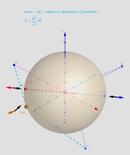
This applet demonstrates how the geometric centers on a sphere change when points are moved in three-dimensional space. Key mathematical concepts include geometric transformations, vectors, and solid geometry. The construction uses GeoGebra commands such as Polygon, PointIn, Sphere, Vector, etc. Suitable for high school and above students or teachers.
GeoGebra Commands & Parameters
Polygon({B01, B02, B04, B03}) → q2PointIn(q2) → B1PointIn(q2) → B2PointIn(q2) → B3PointIn(q2) → B4PointIn(q2) → B5PointIn(q2) → B6PointIn(q2) → B7PointIn(q2) → B8PointIn(q2) → B9PointIn(q2) → B10First({P1, P2, P3, P4, P5, P6, P7, P8, P9, P10}, n) → lPPolygon({((-π), ((-π)) / 2), ((-π), π / 2), (π, π / 2), (π, ((-π)) / 2)}) → qPointIn(q) → A_2Sphere(O, R) → bCircle(O, R, xOyPlane) → cAngle(sumunitA_q, vA) → αAZip(Segment[A, p], p, lP) → segSum(seg) → sum_segPolyLine({((-π), ((-π)) / 2), ((-π), π / 2), (π, π / 2), (π, ((-π)) / 2), ((-π), ((-π)) / 2)}) → q1Flatten(Sequence[Sequence[((-π) + ((2 * π / na) * i), ((-π)) / 2 + (π / na * j)), j, 1, na - 1], i, 1, na - 1]) → ltest_2Zip((R; x(a); y(a)), a, ltest_2) → ltest_3Zip((arg(a), alt(a)), a, lP) → lP_2Textfield(n) → InputBox11KeepIf(x > 0, Sequence[If[abs(Element[αsad, i] - π) < 0.001 ∨ abs(Element[αsad, i]) < 0.001, i, 0], i, 1, Length[αsad]]) → NαsadTextfield(R) → InputBox1Textfield(na) → InputBox2Function(f01, (-π), π, ((-π)) / 2, π / 2) → f0Sequence(Vector[(1.3 * Point[O, Vector[Element[sumunit_sad, i]]]), (1.5 * Point[O, Vector[Element[sumunit_sad, i]]])], i, 1, Length[sumunit_sad]) → sumunit_sad1Zip((Length[a]; arg(a); alt(a)), a, lP) → lPsphereCurveCartesian((-π) + ((2 * π) * a), ((-π)) / 2, f0((-π) + ((2 * π) * a), ((-π)) / 2), a, 0, 1) → par1CurveCartesian((-π) + ((2 * π) * a), π / 2, f0((-π) + ((2 * π) * a), π / 2), a, 0, 1) → par2CurveCartesian(π, ((-π)) / 2 + (π * a), f0(π, ((-π)) / 2 + (π * a)), a, 0, 1) → par4Zip(Text["d_{" + (a) + "}", (A + Element[lP, a]) / 2], a, 1…n) → lPtxtCurveCartesian((-π), ((-π)) / 2 + (π * a), f0((-π), ((-π)) / 2 + (π * a)), a, 0, 1) → par3Zip((x(a), y(a)), a, lP) → lP_{Gr1}First({aP1, aP2, aP3, aP4, aP5, aP6, aP7, aP8, aP9, aP10}, n) → OutputVector((1.3 * A), (1.5 * A)) → lvA_aZip(Segment[F_o, p], p, lP) → segF_oSum(segF_o) → sum_segFoSum(seg^(2)) → sum_qVector((1.3 * A), (1.1 / 1.7 * Point[O, Vector[(-sumunitA_q)]])) → l1A_qVector((1.3 * Zq), (1.5 * Zq)) → lvZqVector((1.3 * Zq'), (1.5 * Zq')) → lvZq'Vector((1.3 * Zq), (1.1 / 1.7 * Point[O, Vector[(-sumunitZ_q)]])) → l1Z_qVector((1.3 * Zq'), (1.1 / 1.7 * Point[O, Vector[(-sumunitZ_q')]])) → l1Z_q'Segment(Zq, Zq') → antipodalAchseSegment(Zq, Cm_0) → segZqSegment(Zq', Cm_0) → segZq'Zip(Segment[Cm_0, p], p, lP) → segC_mSum(Zip[a^(2), a, segC_m]) → sum_segCmoqZip(Text["P_{" + (a) + "}", b + (0.1, 0.1)], a, 1…n, b, lP_2) → l1Zip(Segment[(x(a), y(a), -1), (x(a), y(a), f0(x(a), y(a)))], a, {((-π), ((-π)) / 2), ((-π), π / 2), (π, π / 2), (π, ((-π)) / 2)}) → lsegTranslate(q, Vector[(0, 0, -1)]) → q'RotateText(txt, 90°) → txt1Zip(Segment[AA_2, a], a, alP) → l2
AI Drawing Prompt Reference
Draw a sphere in 3D space with its center at the origin and adjustable radius. Place a quadrilateral plane region inside or on the sphere, and generate several random points within this region. From the sphere's center, draw vectors to each of these points, then compute the sum of these vectors. Based on the direction of the sum vector, mark corresponding points on the sphere's surface and connect them with line segments. Additionally, draw a latitude-longitude grid on the sphere and show an input box to adjust the number of points. Finally, display the points, vectors, sum vector, and their projections on the sphere.
The prompt above was compiled from the original drawing commands and is for reference only.