
GeoGebra Systems of Linear Equations Exploration
Loading the math board and drawing, please wait…
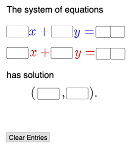
This example dynamically demonstrates the relationship between solution sets and graph images of linear equations. It involves core math concepts like linear equations, function graphs, analytical geometry, and equation solving. Constructed using GeoGebra commands/objects such as Textfield, Mode, If for dynamic parameter adjustment and conditional logic. Suitable for high school mathematics teaching to understand the geometric meaning of solutions to linear systems and the impact of parameter changes.
GeoGebra Commands & Parameters
Textfield(a) → i1Textfield(b) → i2Textfield(c) → i3Textfield(d) → i5Textfield(e) → i6Textfield(f) → i7Textfield(g) → i9Textfield(h) → i9aTextfield(i) → i4Textfield(j) → i8Mode(l1) → l2If(Length[l2] ≟ 0, "No digits repeat.", "Repeated digits exist.") → text2
AI Drawing Prompt Reference
Draw two lines, one defined by the equation ax+by=c and the other by dx+ey=f. Use sliders to adjust the values of a, b, c, d, e, and f, and observe how they affect the position of the lines and their intersection point. By changing the parameters, explore the relationship between the solution set of linear systems and their graphical representations.
The prompt above was compiled from the original drawing commands and is for reference only.