GeoGebra Simulation of Coin-Toss Probability

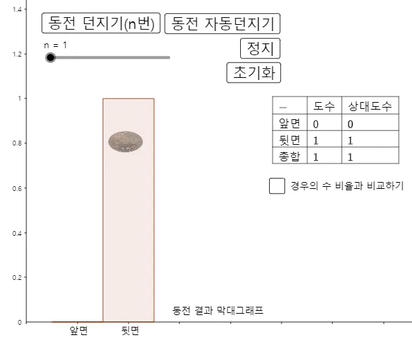
This example demonstrates how coin-toss outcomes change under repeated trials by visualizing the evolving frequencies and the resulting empirical distribution. It focuses on key probability & statistics ideas: random experiments, sample frequency, and how an empirical distribution (Bernoulli-like outcomes) can be observed through repeated simulation. Construction-wise, GeoGebra uses Random to generate coin results, Element to build and manage the results list, Frequency to count occurrences, and Histogram to display those counts as a chart. TableText is used to present summary statistics in a table, while controls such as buttons and the parameter n (number of trials) update the simulation and graphics dynamically. Suitable for middle/high school probability lessons and for exploratory activities on “frequency tends to stabilize with larger samples.”