
GeoGebra Interactive Demo: Solving Simple Linear Equations
Loading the math board and drawing, please wait…
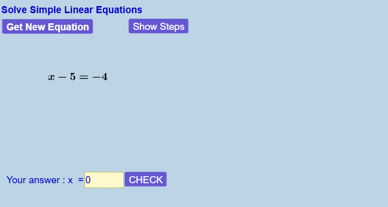
This example demonstrates how to dynamically solve linear equations in GeoGebra through interactive operations, showing the complete process of equation solving. Core mathematical concepts include: solving first-degree equations, substitution elimination method, and the equivalence of performing operations on both sides of an equation. Construction details: Use Random and RandomElement commands to generate equations randomly, extract coefficients with the Coefficients command, implement conditional logic with If commands, dynamically display solving steps via Textfield and Text objects, and simplify expressions using the Simplify command. Objects include: input box for user answers, buttons to control the workflow, text objects to display equations and steps, and variables to store equation parameters. Suitable for middle school mathematics teaching, serving as an interactive demonstration tool to help students understand the logical steps of equation solving.
GeoGebra Commands & Parameters
Random(1, 10) → r_{oo}Element({-5, -4, -3, -2, -1, 1, 2, 3, 4, 5, 6}, r_{oo}) → r0If(count < startbothsidesx, If[count < 2, 1, If[count < 3, RandomElement[{2, -2}], RandomElement[{-3, -2, 2, 3}]]], RandomElement[{-9, -8, -7, -6, -5, -4, -3, -2, -1, 1, 2, 3, 4, 5, 6, 7, 8, 9, 10, 11, 12}]) → r1RandomElement({-9, -8, -7, -6, -5, -4, -3, -2, -1, 1, 2, 3, 4, 5, 6, 7, 8, 9, 10, 11, 12}) → r2If(count < startbothsidesx, If[count < startrightsidex, 0, (-r1)], RandomElement[{-9, -8, -7, -6, -5, -4, -3, -2, -1, 1, 2, 3, 4, 5, 6, 7, 8, 9, 10, 11, 12}]) → r3Simplify(g_3(x) + If[Element[listEqn1LCoeff, 1] < 0, (abs(Element[listEqn1LCoeff, 1]) * x), ((-abs(Element[listEqn1LCoeff, 1])) * x)]) → g_{2s}Simplify(f_3(x) + If[Element[listEqn1LCoeff, 1] < 0, (abs(Element[listEqn1LCoeff, 1]) * x), ((-abs(Element[listEqn1LCoeff, 1])) * x)]) → f_{2s}If(showsteps ≟ true, 10 - display, 1) → stepTextfield(answerx) → inputBox1AnswerIf(answerx ≟ g(0), 1, 0) → correctIf(showsteps ≟ true, 10, 1) → stepsvalueTextfield(operatebothsidesvalue) → inputBox2OperatebothsidesvalueIf(Element[listEqn1LCoeff, 1] < Element[listEqn1RCoeff, 1], true, false) → sSimplify(g_{2s}(x) + If[Element[listEqn1RCoeff, 2] < 0, abs(Element[listEqn1RCoeff, 2]), (-abs(Element[listEqn1RCoeff, 2]))]) → g_{1s}Simplify(f_{2s}(x) + If[Element[listEqn1RCoeff, 2] < 0, abs(Element[listEqn1RCoeff, 2]), (-abs(Element[listEqn1RCoeff, 2]))]) → f_{1s}Coefficients(g_{2s}) → listEqn2RCoeffSLength(listEqn2RCoeffS) → lengthlistEqn2RCoeffCoefficients(f_{2s}) → listEqn2LCoeffSLength(listEqn2LCoeffS) → lengthlistEqn2LCoeffElement(listEqn2RCoeffS, lengthlistEqn2RCoeff) → r2SIf(abs(r1) ≟ 1, true, false) → skip7on
AI Drawing Prompt Reference
Draw a simple process of solving a linear equation, including a randomly generated equation, coefficients, step-by-step solution, and an answer input box. Start by generating a random coefficient, then create the left and right sides of the equation based on the coefficient. Show each step of solving the equation, such as adding, subtracting, multiplying, or dividing both sides, and finally display whether the user's answer is correct.
The prompt above was compiled from the original drawing commands and is for reference only.