
Function Machine by Lew W. S.
Loading the math board and drawing, please wait…
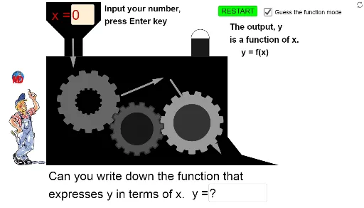
This interactive example demonstrates a function calculator where users input numbers, the machine calculates and displays results, guiding users to guess the function mode. Core math concepts include functions, linear functions, normal distribution, division, random experiments, tangent lines, and similar triangles. It is constructed using GeoGebra commands like CurveCartesian, Circle, Polygon, Point, Textfield, Vector, Semicircle, Mod, Segment, LaTeX, etc. Suitable for high school mathematics teaching to understand and explore function concepts.
GeoGebra Commands & Parameters
CurveCartesian(x(A) + ((r * (a + (1 / b * tanh((b * sin((n * t) + v)))))) * cos(t + v)), y(A) + ((r * (a + (1 / b * tanh((b * sin((n * t) + v)))))) * sin(t + v)), t, 0, 6.28319) → cCurveCartesian(x(B) + ((R * (a + (1 / b * tanh((b * sin((n * t) - v)))))) * cos(t - v)), y(B) + ((R * (a + (1 / b * tanh((b * sin((n * t) - v)))))) * sin(t - v)), t, 0, 6.28319) → dCircle(B, R + 0.9) → eCircle(A, r + 0.9) → gCircle(A, r + 0.9) → hCurveCartesian(x(A) + ((r * (a + (1 / b * tanh((b * sin((n * t) + v)))))) * cos(t + v)), y(A) + ((r * (a + (1 / b * tanh((b * sin((n * t) + v)))))) * sin(t + v)), t, 0, 6.28319) → iCurveCartesian(x(C) + ((R * (a + (1 / b * tanh((b * sin((n * t) - v)))))) * cos(t - v)), y(C) + ((R * (a + (1 / b * tanh((b * sin((n * t) - v)))))) * sin(t - v)), t, 0, 6.28319) → jCurveCartesian(x(C) + ((r / 2 * (a + (1 / b * tanh((b * sin((n * t) + v)))))) * cos(t + v)), y(C) + ((r / 2 * (a + (1 / b * tanh((b * sin((n * t) + v)))))) * sin(t + v)), t, 0, 6.28319) → oPolygon(D, E, F, G) → poly1, d_1, e_1, f_1, g_1Point(g_1) → HPoint(g_1) → IPolygon(H, I, J, K) → poly2, h_1, i_1, j_1, kPolygon(L, K, J, M) → poly3, l, k_1, j_2, mPoint(f_1) → NPolygon(N, O, P, F) → poly4, n_1, o_1, p, f_2Textfield(s) → ChampTexte1Vector(Q, S) → uTextfield(f) → ChampTexte2Vector(U, V) → wVector(W, Z) → zPolygon(C_1, M, L, D_1) → poly5, c_1, m_1, l_1, d_2Polygon(E_1, F_1, G_1, H_1) → poly6, e_2, f_3, g_2, h_2Semicircle(F_1, G_1) → qMod(v / °, 2) → t_1Semicircle(F_1, G_1) → p_1Segment(A_1, B_1) → a_1LaTeX(f) → textFromFunctionTextToUnicode(textFromFunction) → L_3Text("(" + s + ")") → textFormulaValueTextToUnicode(textFormulaValue) → L_nRemove(Insert[L_n, L_3, IndexOf[120, L_3]], {120}) → L_4Remove(Insert[L_n, L_4, IndexOf[120, L_4]], {120}) → L_5Remove(Insert[L_n, L_5, IndexOf[120, L_5]], {120}) → L_6Remove(Insert[L_n, L_6, IndexOf[120, L_6]], {120}) → L_7Remove(Insert[L_n, L_7, IndexOf[120, L_7]], {120}) → L_8Remove(Insert[L_n, L_8, IndexOf[120, L_8]], {120}) → L_9RemoveUndefined({L_3, L_4, L_5, L_6, L_7, L_8, L_9}) → L_{10}Element(L_{10}, Length[L_{10}]) → L_{11}LaTeX("= " + (UnicodeToText[L_{11}]), true) → textEnumFunctionTextfield(textuserinputfunction) → InputBox1
AI Drawing Prompt Reference
Draw a function calculator illustration featuring two rotating function curves, a large circle and two smaller circles for the machine body, multiple polygons forming the operational interface, points marking key positions, text boxes for input and output, vectors indicating directions, semicircles, and segments for decoration, embodying function computation and geometric construction concepts.
The prompt above was compiled from the original drawing commands and is for reference only.