
Fourier Transform
Loading the math board and drawing, please wait…
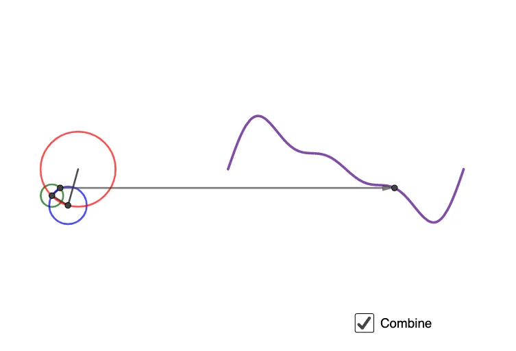
This example demonstrates the process of Fourier Transform, a mathematical method that decomposes signals into different frequencies of sine waves. Using GeoGebra commands such as Circle, Vector, If, Segment, PolyLine, etc., the decomposition process is dynamically displayed. Suitable for university mathematics and signal processing courses.
GeoGebra Commands & Parameters
Circle(A2, R3) → c3Vector(A1, P1) → v1Vector(A2, P1) → v2Vector(A3, P1) → v3If(n ≟ 1, v1, Vector[If[n ≟ 2, v2, v3]]) → vCircle((-4, -2.5), R1) → d1Circle((-4, -4.5), R2) → d2Circle((-4, -6.5), R3) → d3Segment(Center[d1], B1) → b1Segment(Center[d2], B2) → b2Segment(Center[d3], B3) → b3Vector(B1, (t, f1(t))) → u1Vector(B2, (t, f2(t))) → u2Vector(B3, (t, f3(t))) → u3Circle((x(A1), y(A1)), R2) → c2Circle((-4, -4.5), R1) → c1PolyLine((-4, -4.5), A1, A2, A3) → pVector((-4, -4.5), ((-4, -4.5) * (1 - sep)) + (sep * A1)) → vs2Translate(d2, vs2) → c20Vector((-4, -6.5), ((-4, -6.5) * (1 - sep)) + (sep * A2)) → vs3Translate(d3, vs3) → c30Vector((-4, -2.5), (-4, (-4.5 * sep) + ((1 - sep) * (-2.5)))) → vs1Vector((-4, -2.5), (-4, (-4.5 * sep) + ((1 - sep) * (-2.5)))) → vs10Translate(f1, vs10) → ff1Vector((-4, -6.5), (-4, (-4.5 * sep) + ((1 - sep) * (-6.5)))) → vs30Translate(d1, vs1) → c10Translate(f3, vs30) → ff3