
First Fundamental Theorem of Calculus Visualization
Loading the math board and drawing, please wait…
In collections
Fun with Functions
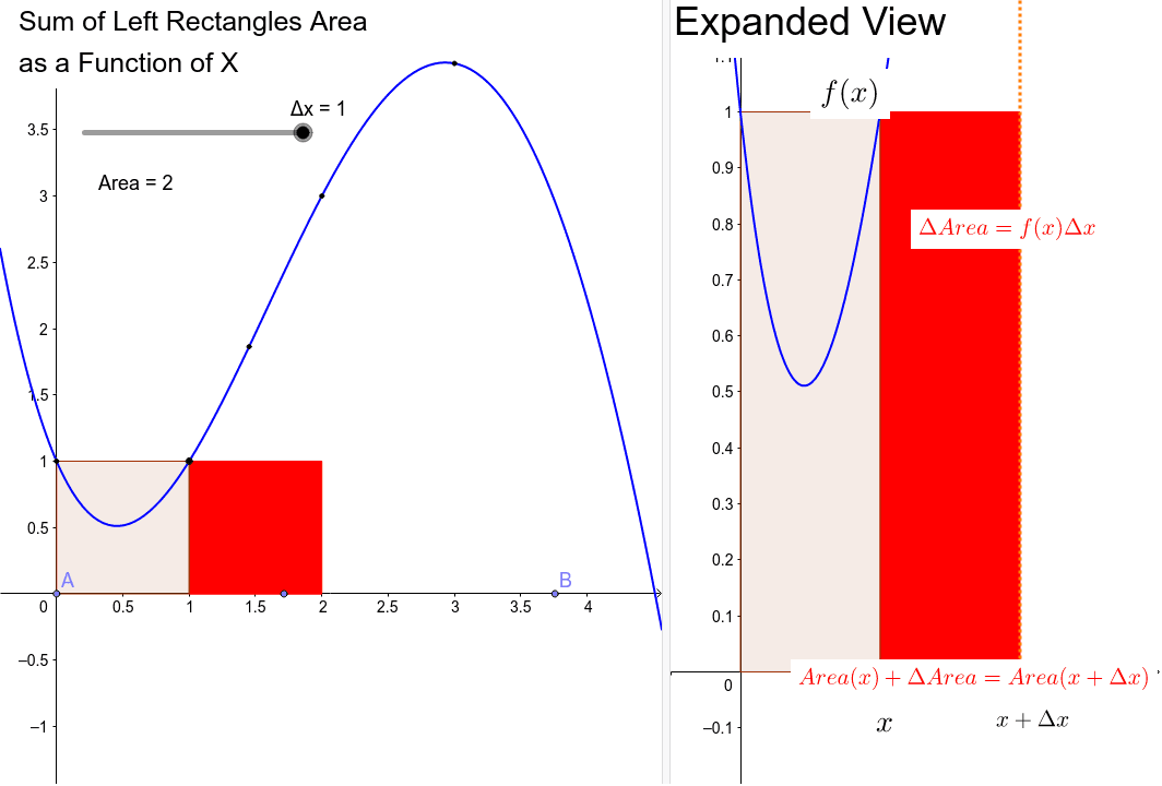
This example visually demonstrates the First Fundamental Theorem of Calculus, illustrating how the area under a curve corresponds to the antiderivative of the function. It involves core concepts like definite integrals, antiderivatives, function graphs, and geometric area calculation. GeoGebra commands used include Polynomial, Point, LeftSum, Defined, Integral, Polygon, and Segment. Suitable for high school students and beginners in calculus learning.
GeoGebra Commands & Parameters
Polynomial({C, D, E, F, G}) → gPoint(xAxis) → APoint(xAxis) → PLeftSum(g, x(A), end, n) → aDefined(a) → cPoint(xAxis) → BIntegral(g, x(A), x(B)) → intergralPolygon({(end, 0), (end, g(end)), (end + Δx, g(end)), (end + Δx, 0)}) → poly1If(c, a + (g(end) * Δx), (g(end) * Δx)) → areaPoint({end + dx, 0}) → xpPoint({end + dx, g(end + dx)}) → fpSegment(xp, fp) → bIf(g(end) > 0, ((-0.2) * g(end)), (1.2 * g(end))) → exBotIf(g(end) > 0, (1.2 * g(end)), ((-0.2) * g(end))) → exTop
AI Drawing Prompt Reference
Draw a function graph and demonstrate the correspondence between the definite integral and the antiderivative. Take two points on the curve, connect them, and calculate the area under the curve. Represent the area with a polygon and connect key points with line segments. Add auxiliary lines and arrows to emphasize the geometric meaning.
The prompt above was compiled from the original drawing commands and is for reference only.