
Extreme Point Distribution on a Sphere: Vector-Based Optimization Visualization
Loading the math board and drawing, please wait…
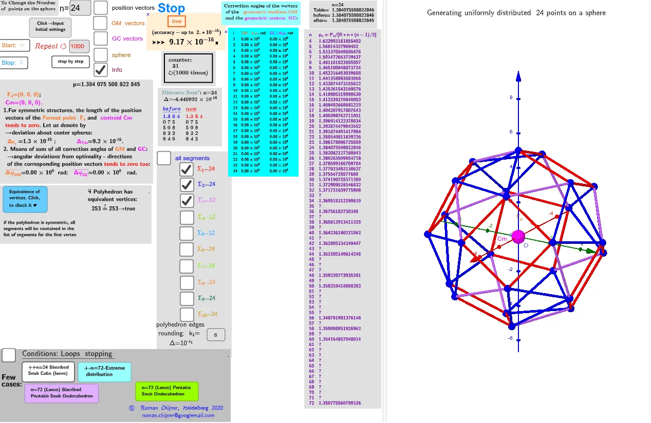
This GeoGebra example demonstrates how to construct and study an “extreme” distribution of points on the surface of a sphere, highlighting how different spherical point configurations affect a chosen objective (e.g., uniformity or spread) and reveal optimal or worst-case patterns. The key math concepts include sphere geometry (Sphere and its surface), 3D vectors, centroid/barycenter ideas to capture average/symmetry properties, and optimization modeling (Optimization Problems) to define objective and constraints that evaluate the distribution quality. Construction details extracted from the command summary show the use of Text and LaTeX for mathematical labels, Sphere to generate the 3D sphere, Textfield for interactive inputs/parameters, and TableText/Append to organize computed values. Logic and aggregation are handled via If and Zip, while Sum is used to accumulate the objective/constraint expressions across points. The setup also reflects parametrization through InputBox1/InputBox2 and variables such as r, n, and related computed quantities (e.g., matrix/mean-like intermediates). The example suits advanced high school through undergraduate learners interested in geometry-based optimization, discrete point placement on manifolds, and interactive mathematical visualization.
GeoGebra Commands & Parameters
Text("" + Um1) → txt_pLaTeX(Um1) → lll1_1LaTeX(Um0) → lll0Sphere(O, R) → p1Textfield(n) → InputBox1Textfield(i0) → InputBox2Text(r) → TxtrTextfield(k_1) → InputBox4UnicodeToLetter(34) → u34Textfield(k_2) → InputBox5TableText(ltxt0, ltxt1, "v") → textltxt01Append(A, Sequence[((random(), random(), random()) * R), i, 2, n]) → l2sText(("(up\; to\; 10^{-15})\;\\ accuracy= " * ScientificText[cc, 3]), C, true, true) → text5rZip(Vector[a, a + UnitVector[a]], a, lP') → lVector1Textfield(scale) → InputBox6TableText(Append["i", 1…n], Append[" \fgcolor{orange}{GM :Δφ_i}, rad", l1], Append["\fgcolor{magenta}{GC :Δφ_i} , rad", l1c], "v") → text23If(bu, "Animation", "Stop") → bue0Zip(Vector[a, a + (1.5 * UnitVector[b])], a, lP', b, Wi_P) → lVector3Zip(Vector[a, a + (1.5 * UnitVector[b])], a, lP', b, Wi_Pc) → lVector2TableText({Join[{{"n"}, Sequence[i, i, 4, 69 + 3]}], Join[{{" p_n=P_n/[R*n*(n-1)/2]"}, lp}]}, "vl") → txt_lpSum(Flatten[Sequence[Append[Sequence[Element[txt_p, i], i, m1(k), m2(k)], " "], k, 1, 5]]) → txtUm1Zip(Segment[Element[lP', y(a)], Element[lP', z(a)]], a, ll1bb(1)) → ll1Zip(Segment[Element[lP', y(a)], Element[lP', z(a)]], a, ll1bb(2)) → ll2Zip(Segment[Element[lP', y(a)], Element[lP', z(a)]], a, ll1bb(3)) → ll3Zip(Segment[Element[lP', y(a)], Element[lP', z(a)]], a, ll1bb(4)) → ll4Zip(Segment[Element[lP', y(a)], Element[lP', z(a)]], a, ll1bb(5)) → ll5Zip(Segment[Element[lP', y(a)], Element[lP', z(a)]], a, ll1bb(6)) → ll6Zip(Segment[Element[lP', y(a)], Element[lP', z(a)]], a, ll1bb(7)) → ll7Zip(Segment[Element[lP', y(a)], Element[lP', z(a)]], a, ll1bb(8)) → ll8Zip(Segment[Element[lP', y(a)], Element[lP', z(a)]], a, ll1bb(9)) → ll9Zip(Segment[Element[lP', y(a)], Element[lP', z(a)]], a, ll1bb(10)) → ll10Text("\;\;\;\;\;\;\;\;\;\;\;\;\;\fgcolor{" + (If[c', "orange", "brown"]) + "} \boxed{ " + c' + ("}\;\;\;\; \;\;\;\;\; \\\;\; ( accuracy- up\; to\;\; 2.*10^{" - k_2) + ("\;})\;\\\;\; ➤➤➤\;\;\;\scalebox{1.5}{ " + (ScientificText[cc, 3])) + "}\;█ ", C, true, true) → text9
AI Drawing Prompt Reference
Visualize a sphere with randomly distributed points on its surface. For each point, draw vectors from the sphere's center to the points, with varying colors and thicknesses. Label the sphere's radius, number of points, and vector information for each point. Also, display the analysis results of the points' distribution uniformity.
The prompt above was compiled from the original drawing commands and is for reference only.